Signal Uncertainties#
A walk-through of how the simplified-likelihood backends in Spey use signal-side systematic uncertainties through log-normal morphing, with numerical examples on a two-bin model.
Introduction#
Hypothesis tests in collider searches rest on the profile likelihood ratio \(\lambda(\mu) = \mathcal{L}(\mu, \hat{\hat{\boldsymbol{\theta}}})/\mathcal{L}(\hat\mu, \hat{\boldsymbol{\theta}})\), where the nuisance parameters \(\boldsymbol{\theta}\) are profiled out at every value of the parameter of interest \(\mu\). Background systematics — luminosity, jet energy scale, MC statistics — are commonly absorbed into \(\boldsymbol{\theta}\) via Gaussian constraint terms. Signal systematics (theory-cross-section, PDF, QCD-scale, acceptance) play exactly the same role: they shift the predicted signal yield in each bin and therefore broaden the \(\chi^{2}(\mu)\) profile, which in turn relaxes the upper limit on \(\mu\).
Spey exposes signal uncertainties through the modifiers keyword of the
default.* backends. Each modifier introduces additional nuisance parameters
with standard-normal priors and a multiplicative log-normal morphing of the
nominal signal yield. This notebook derives the modified likelihood for every
supported modifier type and demonstrates the numerical impact on a two-bin
toy.
Likelihood structure without signal uncertainties#
For the uncorrelated-background backend (default.uncorrelated_background) the
likelihood factorises over \(N\) statistically independent bins,
with the expected count in bin \(i\)
Symbol dictionary:
Symbol |
Meaning |
|---|---|
\(\mu\) |
signal-strength parameter of interest (POI) |
\(n^{(s)}_i\) |
nominal signal yield in bin \(i\) |
\(n^{(b)}_i\) |
nominal background yield in bin \(i\) |
\(\sigma_i\) |
absolute background uncertainty in bin \(i\) |
\(\theta_i\) |
background nuisance parameter for bin \(i\) (standard-normal prior) |
\(n^{\mathrm{obs}}_i\) |
observed event count in bin \(i\) |
The test statistic for upper limits is
where \(\hat\mu, \hat{\boldsymbol{\theta}}\) are the global maximum-likelihood estimators and \(\hat{\hat{\boldsymbol{\theta}}}(\mu)\) are the conditional MLEs at fixed \(\mu\). Throughout this notebook we plot the symmetric profile \(\Delta\chi^{2}(\mu) = -2\bigl[\ln\mathcal{L}(\mu,\hat{\hat{\boldsymbol{\theta}}}(\mu)) - \ln\mathcal{L}(\hat\mu,\hat{\boldsymbol{\theta}})\bigr]\), which under Wilks’ theorem is asymptotically \(\chi^{2}_{1}\)-distributed and crosses \(3.84\) at the two-sided \(95\,\%\) confidence level.
How signal uncertainties modify the likelihood#
Spey implements signal systematics via log-normal morphing of the nominal signal yield. For an uncertainty source \(k\) with per-bin absolute variation \(\sigma^{(s)}_{i,k}\), define the per-bin fractional shift
The synthesizer in spey.backends.default_pdf.uncertainty_synthesizer exposes
two modifier types, selected via the "type" key of each modifier dictionary.
Each modifier also accepts a "name" (used for parameter labelling) and
"uncertainties" (per-bin absolute values; a flat list[float] for symmetric
uncertainties or a list[(up, down)] for asymmetric ones).
"type": "shape" — one nuisance per bin#
Each bin receives its own independent nuisance \(\alpha_{i,k}\), with morphing factor
The likelihood gains \(N\) independent standard-normal constraint factors:
This is the right choice when an uncertainty distorts the shape of the distribution — bin-by-bin scale-variation envelopes, MC-statistical errors on theory templates, or any source whose bins are not coherently correlated.
Multiple sources combine multiplicatively#
When several modifiers are stacked the per-bin signal modifier is the product of the individual factors:
and the constraint term is a product of independent standard-normal priors —
one per shared normalization nuisance, \(N\) per shape modifier. The Poisson
term does not factorise over modifiers because they all multiply the same
\(\mu\, n^{(s)}_i\), but the constraint term does.
Bins with \(n^{(s)}_i = 0\) produce \(\Delta_{i,k} = \mathrm{NaN}\); the synthesizer replaces those with \(1\) so the morphing factor is identically \(1\) in those bins.
Which backends accept signal uncertainties#
The four default.* simplified-likelihood backends all accept the
modifiers keyword and route it through the same
signal_uncertainty_synthesizer. The cell below introspects every backend
registered with spey.AvailableBackends() and reports whether the
constructor signature exposes a modifiers parameter.
| backend | accepts_modifiers | |
|---|---|---|
| 0 | default.correlated_background | True |
| 1 | default.effective_sigma | True |
| 2 | default.multivariate_normal | False |
| 3 | default.normal | False |
| 4 | default.poisson | False |
| 5 | default.third_moment_expansion | True |
| 6 | default.uncorrelated_background | True |
| 7 | hs3 | False |
| 8 | pyhf | False |
| 9 | pyhf.simplify | False |
| 10 | pyhf.uncorrelated_background | False |
All four default.* simplified-likelihood backends — uncorrelated_background,
correlated_background, third_moment_expansion, and effective_sigma —
share the same modifiers plumbing. Backends that wrap an external
model-building framework (e.g. the pyhf.* family) carry their own
systematics machinery and do not expose this keyword.
Baseline model#
We work with a two-bin counting experiment in which both bins exhibit a downward fluctuation relative to the background-plus-nominal-signal prediction.
pdf_wrapper = spey.get_backend("default.uncorrelated_background")

baseline_model = pdf_wrapper(
    signal_yields=[12.0, 15.0],
    background_yields=[50.0, 48.0],
    data=[36, 33],
    absolute_uncertainties=[12.0, 16.0],
)

print(f"backend            : {baseline_model.backend_type}")
print(f"chi2(mu = 1)       : {baseline_model.chi2(poi_test=1.0):.4f}")
print(f"95% CL mu upper    : {baseline_model.poi_upper_limit():.4f}")
backend            : default.uncorrelated_background
chi2(mu = 1)       : 4.9138
95% CL mu upper    : 0.8563
Adding signal uncertainties#
The next three subsections build a variant of the baseline model with each modifier type in turn, then a combined variant that stacks both. All variants share the same observed data and background model, only the signal-side constraint structure changes.
Normalization modifier: PDF-style coherent variation#
PDF-eigenvector variations (PDF4LHC prescription) move the inclusive cross-section coherently across the kinematic spectrum. A single nuisance parameter therefore captures the bulk of the effect. Here we apply a \(15\,\%\) relative PDF uncertainty to each bin, which corresponds to \(1.8\) and \(2.25\) events in absolute terms (\(0.15 \times 12\) and \(0.15 \times 15\)).
# 15% relative PDF uncertainty per bin -> absolute values of 0.15 * n_s_i.
norm_model = pdf_wrapper(
    signal_yields=[12.0, 15.0],
    background_yields=[50.0, 48.0],
    data=[36, 33],
    absolute_uncertainties=[12.0, 16.0],
    modifiers=[
        {"type": "normalization", "name": "pdf", "uncertainties": [1.8, 2.25]},
    ],
)

print(f"baseline chi2(mu=1) : {baseline_model.chi2(poi_test=1.0):.4f}")
print(f"normalization chi2  : {norm_model.chi2(poi_test=1.0):.4f}")
baseline chi2(mu=1) : 4.9138
normalization chi2  : 4.7284
Shape modifier: bin-by-bin scale variation#
QCD scale variations (\(\mu_R, \mu_F\) rescaled by conventional factors of two)
behave differently from PDFs: the envelope is bin-dependent because
higher-order corrections grow with the event hardness. A shape modifier with
asymmetric (up, down) values mirrors the asymmetric envelopes typically
tabulated by NLO generators. Here we use \(\pm 20\,\%\) in bin 0 and
\(\pm 25\,\%\) in bin 1 with a \(\sim 5\,\%\) up/down asymmetry to imitate
a real scale envelope.
# Asymmetric (up, down) absolute uncertainties per bin.
# Bin 0: +20% / -15% on n_s = 12  ->  (+2.4, -1.8)
# Bin 1: +25% / -20% on n_s = 15  ->  (+3.75, -3.0)
shape_model = pdf_wrapper(
    signal_yields=[12.0, 15.0],
    background_yields=[50.0, 48.0],
    data=[36, 33],
    absolute_uncertainties=[12.0, 16.0],
    modifiers=[
        {
            "type": "shape",
            "name": "scale",
            "uncertainties": [(2.4, 1.8), (3.75, 3.0)],
        },
    ],
)

print(f"baseline chi2(mu=1) : {baseline_model.chi2(poi_test=1.0):.4f}")
print(f"shape    chi2(mu=1) : {shape_model.chi2(poi_test=1.0):.4f}")
baseline chi2(mu=1) : 4.9138
shape    chi2(mu=1) : 4.7881
Combined modifiers: PDF and scale together#
A realistic theory uncertainty stacks both: a coherent PDF variation plus a bin-dependent scale envelope. As shown in Section 3.3, the morphing factors multiply bin-by-bin while their constraint terms remain independent.
combined_model = pdf_wrapper(
    signal_yields=[12.0, 15.0],
    background_yields=[50.0, 48.0],
    data=[36, 33],
    absolute_uncertainties=[12.0, 16.0],
    modifiers=[
        {"type": "normalization", "name": "pdf", "uncertainties": [1.8, 2.25]},
        {
            "type": "shape",
            "name": "scale",
            "uncertainties": [(2.4, 1.8), (3.75, 3.0)],
        },
    ],
)

print(f"baseline chi2(mu=1) : {baseline_model.chi2(poi_test=1.0):.4f}")
print(f"combined chi2(mu=1) : {combined_model.chi2(poi_test=1.0):.4f}")
baseline chi2(mu=1) : 4.9138
combined chi2(mu=1) : 4.6213
Visualising the effect on the \(\chi^{2}\) profile#
We scan \(\mu \in [0, 3]\) at \(80\) points for every model and plot the profile \(-2\,\Delta\ln\mathcal{L}(\mu) = q_\mu\). The Wilks threshold at \(3.84\) marks the two-sided \(95\,\%\) CL crossing; the loosest model is the one whose curve crosses the threshold furthest to the right.
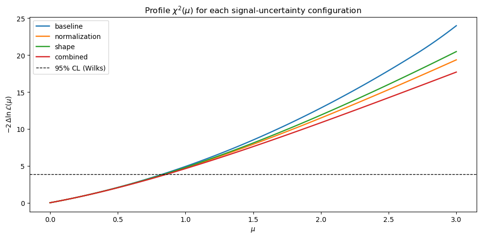
Effect on exclusion limits#
The \(95\,\%\) CL upper limit on \(\mu\) is obtained from
statistical_model.poi_upper_limit(). We tabulate the limit for the baseline
model and every variant together with the relative shift in percent.
| model | upper_limit_mu | delta_vs_baseline_pct | |
|---|---|---|---|
| 0 | baseline | 0.856335 | 0.000000 |
| 1 | normalization | 0.877000 | 2.413259 |
| 2 | shape | 0.870038 | 1.600235 |
| 3 | combined | 0.890584 | 3.999557 |
The combined variant has the largest upper limit on \(\mu\) — both morphing
factors enlarge the allowed signal envelope and the profile likelihood
compensates by accepting a larger \(\mu\) before the data become inconsistent.
Among the single-source variants the normalization modifier produces the
larger shift even though its per-bin variation (\(15\,\%\)) is smaller than the
shape modifier (\(20\)–\(25\,\%\)): a single shared nuisance can pull the signal
down coherently in both bins at a Gaussian penalty of only \(\theta^{2}/2\),
whereas the two independent shape nuisances each pay their own
\(\alpha_{i}^{2}/2\) penalty to achieve the same coherent shift, making the
shape handle stiffer despite its larger nominal envelope.
Summary#
Signal systematics are absorbed by log-normal morphing of the nominal signal yield (\(f_{i,k}(\theta_k) = \exp[\theta_k\ln(1+\Delta_{i,k})]\)), introducing additional nuisance parameters with standard-normal priors.
Pick
"type": "normalization"for sources that move all bins coherently, luminosity, cross-section normalisation, single-eigenvector PDF variations. One nuisance parameter is added.Pick
"type": "shape"for sources whose bin-by-bin effect is uncorrelated, scale envelopes, MC-stat errors on theory templates. One nuisance parameter per bin is added.Multiple modifiers stack multiplicatively in the Poisson term and additively in the log-constraint term; they always inflate the \(\chi^{2}\) profile and therefore relax the upper limit.
All four
default.*simplified-likelihood backends;uncorrelated_background,correlated_background,third_moment_expansion, andeffective_sigma, accept the samemodifierskeyword.