Multi-Parameter Confidence Contours with Spey

This notebook demonstrates how to map multi-dimensional chi-squared confidence contours using the spey.multiparameter sub-package. We work with a two-bin counting experiment whose signal is a linear combination of three benchmark signal shapes, controlled by three free parameters. The goal is to identify the full set of signal-shape parameter combinations that are compatible with the observed data at the 95% confidence level.

The signal strength \(\mu\) is held fixed at 1 throughout. The contour lives in the 3-dimensional space of signal-shape parameters \((c_0, c_1, c_2)\).

---

Contents

1. Theoretical Background

2. Experimental Setup

3. Building the Statistical Model

4. Exploring the Likelihood Landscape

5. Running find_contour

6. Visualising the Confidence Contour

7. Algorithm Walk-through

1 · Theoretical Background

The Statistical Model

We use the multivariate Gaussian likelihood for correlated bins:

\[ \mathcal{L}(\mu,\,c_0,c_1,c_2) = \mathcal{N}\!\bigl(n\,\big|\,\mu\,s(c_0,c_1,c_2)+b,\;\Sigma\bigr), \]

where \(n\) is the observed data, \(b\) the background yields, \(\Sigma\) the covariance matrix, and \(\mu\) the overall signal strength. In this analysis we fix \(\mu = 1\) and let the signal-shape parameters \((c_0, c_1, c_2)\) vary freely.

Wilks’ Theorem and the Confidence Contour

Let \(\theta_s = (c_0, c_1, c_2)\) be the signal-shape parameter vector and \(\hat\theta_s\) its maximum-likelihood estimate (with \(\mu=1\) fixed). Under Wilks’ theorem the test statistic

\[ \chi^2(\theta_s) = 2\bigl[\mathrm{NLL}(\theta_s) - \mathrm{NLL}(\hat\theta_s)\bigr] \]

follows a \(\chi^2_k\) distribution with \(k=3\) degrees of freedom (one per free parameter). The 95% confidence region is

\[ \mathcal{C}_{0.95} = \bigl\{\theta_s : \chi^2(\theta_s) \le \Delta_{0.95}\bigr\}, \qquad \Delta_{0.95} = F^{-1}_{\chi^2_3}(0.95) \approx 7.81. \]

The boundary — the confidence contour — is the 2-dimensional surface satisfying

\[ \mathrm{NLL}(\theta_s) = T, \qquad T = \mathrm{NLL}(\hat\theta_s) + \tfrac{\Delta_{0.95}}{2}. \]

Why fix \(\mu=1\)? In many HEP analyses the signal-shape parameters \((c_0,c_1,c_2)\) encode physical model parameters (e.g. couplings, masses) while \(\mu\) is a nuisance-like overall normalisation. Fixing \(\mu=1\) and profiling the shape parameters gives the confidence region in the physical parameter space of interest.

2 · Experimental Setup

We have a two-bin experiment. The physical signal is a linear combination of three benchmark templates:

\[ s(c_0, c_1, c_2) = c_0\,s_1 + c_1^2\,s_2 + c_2\,s_3, \]

where \(c_1\) enters quadratically — typical when the parameter corresponds to a coupling that appears in the amplitude squared. The total expected yield in each bin is

\[ \lambda = \mu\,s(c_0,c_1,c_2) + b = s(c_0,c_1,c_2) + b \quad (\mu = 1). \]

The three free parameters \((c_0, c_1, c_2)\) define a 3-dimensional signal-parameter space. find_contour maps the 2-dimensional boundary of the 95% CL region in this space.

Show code cell content

Hide code cell content

import warnings

warnings.filterwarnings("ignore")  # suppress minor optimiser warnings for clarity

import numpy as np
import matplotlib.pyplot as plt
from itertools import combinations
from scipy.stats import chi2 as chi2_dist

import spey
from spey.multiparameter import find_contour

print(f"Spey version : {spey.__version__}")
print(f"NumPy version: {np.__version__}")

Spey - WARNING: An unstable version of Spey (0.2.7-b2) is being used. Latest stable version is 0.2.6.
Spey version : 0.2.7-b2
NumPy version: 1.24.4

# ── Observed data ────────────────────────────────────────────────────────────
data = np.array([36, 33])

# ── Background yields and covariance ─────────────────────────────────────────
background_yields = np.array([50.0, 48.0])
covariance_matrix = np.array(
    [[144.0, 13.0], [25.0, 256.0]]  # σ²_0,  Cov(0,1)
)  # Cov(1,0), σ²_1

sigma_b = np.sqrt(np.diag(covariance_matrix))
print(f"Background yields   : {background_yields}")
print(f"Background σ (diag) : {sigma_b}")
print(f"Observed data       : {data}")
print(f"Deficit (data - bkg): {data - background_yields}  (negative → data below bkg)")
print(f"Total Pull (data - bkg) / σ: {sum((data - background_yields)/sigma_b):.3f}")

Background yields   : [50. 48.]
Background σ (diag) : [12. 16.]
Observed data       : [36 33]
Deficit (data - bkg): [-14. -15.]  (negative → data below bkg)
Total Pull (data - bkg) / σ: -2.104

# ── Signal templates ─────────────────────────────────────────────────────────
signal_yields1 = np.array([12.0, 15.0])  # process A
signal_yields2 = np.array([6.0, 16.0])  # process B
signal_yields3 = np.array([20.0, 10.0])  # process C

# ── Parametric signal as a function of shape parameters ──────────────────────
#
#   param = (c0, c1, c2)
#
#   The backend calls  signal_yields(pars[1:])  at every evaluation,
#   where pars = [mu, c0, c1, c2] is the full 4-dim parameter vector.
#   We fix mu=1, so the effective expected yield is s(c0,c1,c2) + bkg.
#
def signal_yields(param: np.ndarray) -> np.ndarray:
    """Combined signal as a function of shape parameters (c0, c1, c2).

    c1 enters quadratically: reflects a squared-coupling dependence
    typical in EFT or BSM amplitude-squared contributions.
    """
    return (
        param[0] * signal_yields1
        + param[1] ** 2 * signal_yields2
        + param[2] * signal_yields3
    )


print("Signal at (c0, c1, c2) = (1, 1, 1) :", signal_yields(np.ones(3)))
print("Signal at (c0, c1, c2) = (0, 0, 0) :", signal_yields(np.zeros(3)))

Signal at (c0, c1, c2) = (1, 1, 1) : [38. 41.]
Signal at (c0, c1, c2) = (0, 0, 0) : [0. 0.]

3 · Building the Statistical Model

We construct a StatisticalModel using the MultivariateNormal backend with n_signal_parameters=3. This tells the backend that the callable signal_yields takes three extra parameters beyond \(\mu\). Internally the backend extends the optimiser parameter vector to

\[ \text{pars} = [\underbrace{\mu}_{\text{index 0 (poi\_index)}},\; \underbrace{c_0,\; c_1,\; c_2}_{\text{indices 1–3}}]. \]

The model knows that index 0 is the POI (\(\mu\)) via cfg.poi_index = 0. find_contour uses cfg.poi_index to:

1. Exclude \(\mu\) from the contour search space.

2. Fix \(\mu=1\) when evaluating the NLL, by passing fixed_poi_value=1.0 to the internal fit() call.

3. Extract the signal-parameter block of the Hessian for the whitening transform.

The resulting contour lives in the 3-dimensional space \((c_0, c_1, c_2)\).

# ── Construct the backend ─────────────────────────────────────────────────────
pdf_wrapper = spey.get_backend('default.multivariate_normal')
stat_model = pdf_wrapper(
    signal_yields=signal_yields,  # callable: (c0, c1, c2) → array[2]
    background_yields=background_yields,
    data=data,
    covariance_matrix=covariance_matrix,
    n_signal_parameters=3,  # declares c0, c1, c2 as free parameters
    analysis="multi_param_demo"
)

print(stat_model)

StatisticalModel(analysis='multi_param_demo', backend=default.multivariate_normal, calculators=['toy', 'asymptotic', 'chi_square'])

# ── Inspect the model configuration ──────────────────────────────────────────
cfg = stat_model.backend.config()
print(f"Total parameters    : {cfg.npar}              (mu + c0 + c1 + c2)")
print(f"All parameter names : {cfg.parameter_names}")
print(f"POI index (mu)      : {cfg.poi_index}")
print()
print("find_contour will fix mu=1 and search for the contour in the")
print(f"  {cfg.npar - 1}-dimensional subspace: {cfg.parameter_names[1:]}")

Total parameters    : 4              (mu + c0 + c1 + c2)
All parameter names : ['mu', 'signal_par_0', 'signal_par_1', 'signal_par_2']
POI index (mu)      : 0

find_contour will fix mu=1 and search for the contour in the
  3-dimensional subspace: ['signal_par_0', 'signal_par_1', 'signal_par_2']

4 · Exploring the Likelihood Landscape

Before running the full contour finder it is instructive to:

1. Locate the MLE of the signal parameters \(\hat\theta_s\) with \(\mu=1\) fixed.

2. Compute the NLL threshold \(T = \mathrm{NLL}(\hat\theta_s) + \Delta_{0.95}^{(k=3)}/2\).

3. Visualise 1-D NLL profiles along each signal-parameter axis.

The MLE is found by calling maximize_likelihood with fixed_poi_value=1.0 (fixes \(\mu=1\) in the optimizer) and poi_indices=[1, 2, 3] (returns \((c_0, c_1, c_2)\) values).

# ── Find the MLE of signal parameters with mu fixed at 1 ─────────────────────
#
#   fixed_poi_value=1.0  →  mu (pars[poi_index]) is pinned to 1
#   poi_indices=[1,2,3]  →  return the fitted values of c0, c1, c2
#
signal_indices = [i for i in range(cfg.npar) if i != cfg.poi_index]  # [1, 2, 3]
signal_names = [cfg.parameter_names[i] for i in signal_indices]  # ['signal_par_0', ...]
k = len(signal_indices)  # = 3

poi_dict, nll_min = stat_model.maximize_likelihood(
    poi_indices=signal_indices,
    return_nll=True,
    fixed_poi_value=1.0,  # fix mu=1; forwarded to fit() via **kwargs
)
theta_mle = np.array([poi_dict[i] for i in signal_indices])  # (c0_hat, c1_hat, c2_hat)

print("MLE of signal parameters (mu=1 fixed):")
for name, val in zip(signal_names, theta_mle):
    print(f"  {name:15s} = {val:+.4f}")
print(f"\nNLL at MLE : {nll_min:.6f}")

MLE of signal parameters (mu=1 fixed):
  signal_par_0    = -1.0792
  signal_par_1    = +0.3634
  signal_par_2    = -0.0921

NLL at MLE : 7.090945

# ── Chi-squared threshold ─────────────────────────────────────────────────────
#
#   DoF = k = 3 (signal-shape parameters only; mu is NOT profiled)
#
delta = chi2_dist.ppf(0.95, df=k)  # Δ_{0.95}^{(k=3)}
threshold = nll_min + delta / 2.0  # NLL threshold T

print(f"Degrees of freedom   : k = {k}  (signal-shape parameters only)")
print(f"Chi-squared quantile : Δ = {delta:.4f}  (at 95% CL, k=3)")
print(f"NLL threshold        : T = {threshold:.6f}")
print()
print("Points θs with  2[NLL(θs) − NLL(θ̂s)] ≤ Δ  lie inside the 95% CR.")

Degrees of freedom   : k = 3  (signal-shape parameters only)
Chi-squared quantile : Δ = 7.8147  (at 95% CL, k=3)
NLL threshold        : T = 10.998309

Points θs with  2[NLL(θs) − NLL(θ̂s)] ≤ Δ  lie inside the 95% CR.

# ── 1-D NLL profiles along each signal-parameter axis ────────────────────────
#
#   We build a reduced NLL function with mu=1 fixed:
#     nll_fixed(signal_pars) = -logpdf([1, signal_pars[0], signal_pars[1], signal_pars[2]])
#
logpdf_fn = stat_model.backend.get_logpdf_func()


def nll_fixed(signal_pars):
    """NLL with mu=1 fixed; takes only the 3 signal-shape parameters."""
    full_pars = np.concatenate([[1.0], signal_pars])  # [mu=1, c0, c1, c2]
    return -float(logpdf_fn(full_pars))


scan_widths = [2.0, 2.0, 1.5]
latex_names = [r"$c_0$", r"$c_1$", r"$c_2$"]

fig, axes = plt.subplots(1, k, figsize=(13, 3.8))
fig.suptitle(r"1-D NLL profiles with $\mu=1$ fixed (others at MLE)", fontsize=13)

for i, (ax, name, width) in enumerate(zip(axes, latex_names, scan_widths)):
    grid = np.linspace(theta_mle[i] - width, theta_mle[i] + width, 120)
    pars_scan = np.tile(theta_mle, (len(grid), 1))
    pars_scan[:, i] = grid
    chi2_vals = 2.0 * (np.array([nll_fixed(p) for p in pars_scan]) - nll_min)

    ax.plot(grid, chi2_vals, color="steelblue", lw=2)
    ax.axvline(
        theta_mle[i],
        color="tomato",
        ls="--",
        lw=1.5,
        label=rf"$\hat{{\theta}}$ = {theta_mle[i]:.3f}",
    )
    ax.axhline(
        delta,
        color="k",
        ls=":",
        lw=1.2,
        label=rf"$\Delta_{{0.95}}^{{(3)}}$ = {delta:.2f}",
    )
    ax.set_xlabel(name, fontsize=12)
    ax.set_ylabel(r"$\chi^2(\theta_s)$", fontsize=12)
    ax.legend(fontsize=8)
    ax.set_ylim(0, delta * 2.5)

plt.tight_layout()
plt.show()

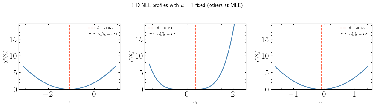
The horizontal dotted line marks \(\Delta_{0.95}^{(k=3)} \approx 7.81\). Each 1-D profile intersection gives a marginal 95% CI for that parameter — but the full multi-dimensional shape can have non-trivial correlations, motivating the 2-D surface mapping.

5 · Running find_contour

find_contour detects cfg.poi_index automatically and:

• Fixes \(\mu=1\) when evaluating the NLL by passing fixed_poi_value=1.0 to the optimizer.

• Builds a reduced NLL \(\mathrm{NLL}(c_0,c_1,c_2)\) using autograd.numpy.concatenate to insert \(\mu=1\) at the correct position — keeping the function fully differentiable for the RATTLE stage.

• Uses the \(3\times 3\) signal-parameter block of the full \(4\times 4\) Hessian for the whitening transform.

• Returns contour points in the 3-D signal-parameter space with DoF = 3 and \(\Delta_{0.95} \approx 7.81\).

Stage	What it does
Pre-whitening	Fisher-information Cholesky in signal space → approximately spherical contour
Radial search	\(N\) random rays + Brent root-finding along each
Gap detection	Cosine-similarity coverage scoring → seed directions
RATTLE HMC	Constrained Hamiltonian chain walking along \(\mathrm{NLL}=T\)

# ── Run the contour finder ────────────────────────────────────────────────────
#
#   find_contour automatically uses cfg.poi_index to exclude mu and
#   fix it at 1.  No manual handling of mu is needed.
#
result = find_contour(
    stat_model,
    confidence_level=0.95,
    n_radial=2000,  # Stage 2: random radial rays
    n_hmc_chains=100,  # Stage 4: RATTLE chains (gap seeds)
    n_hmc_steps=4000,  # Stage 4: leapfrog steps per chain
    hmc_step_size=0.05,  # Stage 4: leapfrog step size ε
    n_gap_candidates=3000,  # Stage 3: candidate directions for gap detection
    random_seed=42,
    bounds=[(-50, 1), (None, None), (None, None)],
    n_jobs=8,
)
print(result)

Running HMC Chain: 8it [00:00, 25.86it/s]

Spey - WARNING: An unstable version of Spey (0.2.7-b2) is being used. Latest stable version is 0.2.6.
Spey - WARNING: An unstable version of Spey (0.2.7-b2) is being used. Latest stable version is 0.2.6.

Running HMC Chain: 16it [00:04,  3.43it/s]

Spey - WARNING: An unstable version of Spey (0.2.7-b2) is being used. Latest stable version is 0.2.6.
Spey - WARNING: An unstable version of Spey (0.2.7-b2) is being used. Latest stable version is 0.2.6.
Spey - WARNING: An unstable version of Spey (0.2.7-b2) is being used. Latest stable version is 0.2.6.
Spey - WARNING: An unstable version of Spey (0.2.7-b2) is being used. Latest stable version is 0.2.6.
Spey - WARNING: An unstable version of Spey (0.2.7-b2) is being used. Latest stable version is 0.2.6.
Spey - WARNING: An unstable version of Spey (0.2.7-b2) is being used. Latest stable version is 0.2.6.

Running HMC Chain: 100it [00:33,  3.02it/s]

ContourResult(theta_mle=array([-1.07916624,  0.36336828, -0.09214556]), nll_min=7.090944826540303, threshold=10.998308778165892, delta=7.8147279032511765, contour_points=array([[ -2.84559878,   1.9755481 ,   0.64245939],
       [  0.55722097,  -1.24603069,  -0.69750495],
       [  0.24860554,  -1.24318741,  -0.38716747],
       ...,
       [-49.9221291 ,  -5.51807397,  20.26939748],
       [-49.95411055,  -5.51889602,  20.32220829],
       [-49.98602794,  -5.51984623,  20.37516206]]), from_radial=array([ True,  True,  True, ..., False, False, False]), parameter_names=['signal_par_0', 'signal_par_1', 'signal_par_2'], confidence_level=0.95, dof=3)

# ── Inspect the ContourResult ─────────────────────────────────────────────────
print("=" * 55)
print("ContourResult summary")
print("=" * 55)
print(f"Confidence level      : {result.confidence_level:.0%}")
print(f"Degrees of freedom    : k = {result.dof}  (signal-shape params only)")
print(f"Chi-squared threshold : Δ = {result.delta:.4f}")
print(f"NLL at MLE (mu=1)     : {result.nll_min:.6f}")
print(f"NLL threshold         : T = {result.threshold:.6f}")
print()
print("Signal-parameter MLE (mu=1 fixed):")
for name, val in zip(result.parameter_names, result.theta_mle):
    print(f"  {name:18s} = {val:+.4f}")
print()
print(f"Total contour points  : {len(result.contour_points)}")
print(f"  From radial search  : {result.from_radial.sum()}")
print(f"  From RATTLE HMC     : {(~result.from_radial).sum()}")

=======================================================
ContourResult summary
=======================================================
Confidence level      : 95%
Degrees of freedom    : k = 3  (signal-shape params only)
Chi-squared threshold : Δ = 7.8147
NLL at MLE (mu=1)     : 7.090945
NLL threshold         : T = 10.998309

Signal-parameter MLE (mu=1 fixed):
  signal_par_0       = -1.0792
  signal_par_1       = +0.3634
  signal_par_2       = -0.0921

Total contour points  : 149249
  From radial search  : 1959
  From RATTLE HMC     : 147290

# ── Verify that contour points satisfy NLL(θs) ≈ T ───────────────────────────
rng_check = np.random.default_rng(0)
check_idx = rng_check.choice(
    len(result.contour_points),
    size=min(40, len(result.contour_points)),
    replace=False,
)

residuals = np.array(
    [nll_fixed(result.contour_points[i]) - result.threshold for i in check_idx]
)

print(f"Spot-check of {len(check_idx)} contour points:")
print(f"  Max  |NLL(θs) − T| = {np.abs(residuals).max():.2e}")
print(f"  Mean |NLL(θs) − T| = {np.abs(residuals).mean():.2e}")
print()
print("All residuals small → points lie on the constraint surface.")

Spot-check of 40 contour points:
  Max  |NLL(θs) − T| = 3.83e-10
  Mean |NLL(θs) − T| = 4.35e-11

All residuals small → points lie on the constraint surface.

6 · Visualising the Confidence Contour

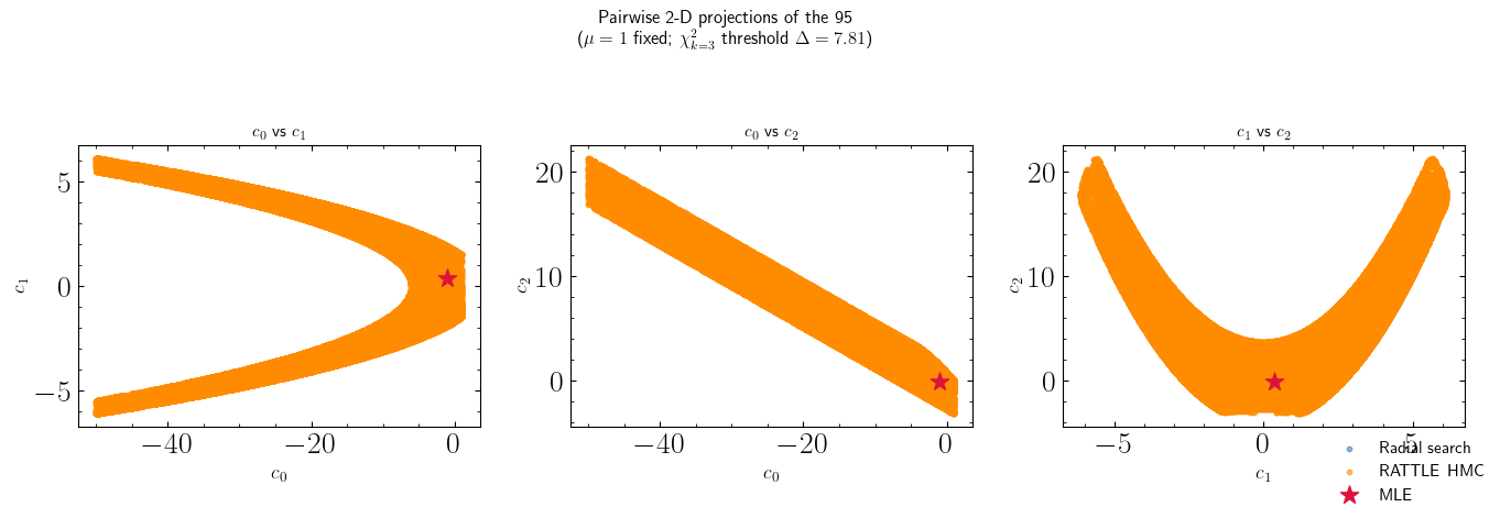
With \(k=3\) signal-shape parameters the confidence contour is a 2-dimensional surface in 3-dimensional space. We show:

• Three pairwise 2-D projections: \((c_0,c_1)\), \((c_0,c_2)\), \((c_1,c_2)\).

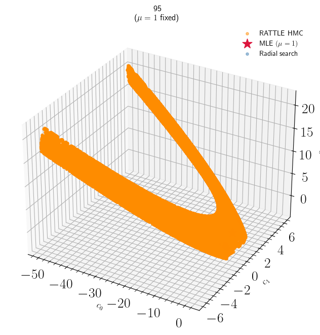
• A 3-D scatter plot of all contour points.

• A residual histogram confirming all points satisfy \(\mathrm{NLL}(\theta_s) \approx T\).

Points are coloured by their origin: blue = radial search, orange = RATTLE HMC. The MLE is the red star.

pts = result.contour_points  # shape (N, 3)
radial_mask = result.from_radial  # bool
mle = result.theta_mle  # (c0_hat, c1_hat, c2_hat)
latex_names = [r"$c_0$", r"$c_1$", r"$c_2$"]

pairs = list(combinations(range(k), 2))  # 3 pairs for k=3

fig, axes = plt.subplots(1, 3, figsize=(14, 4.5))
fig.suptitle(
    "Pairwise 2-D projections of the 95% CL confidence contour\n"
    rf"($\mu=1$ fixed; $\chi^2_{{k=3}}$ threshold $\Delta = {result.delta:.2f}$)",
    fontsize=12,
    y=1.02,
)

for ax, (i, j) in zip(axes, pairs):
    ax.scatter(
        pts[radial_mask, i],
        pts[radial_mask, j],
        s=10,
        alpha=0.6,
        color="steelblue",
        label="Radial search",
    )
    ax.scatter(
        pts[~radial_mask, i],
        pts[~radial_mask, j],
        s=10,
        alpha=0.6,
        color="darkorange",
        label="RATTLE HMC",
    )
    ax.scatter(mle[i], mle[j], s=150, color="crimson", marker="*", zorder=5, label="MLE")
    ax.set_xlabel(latex_names[i], fontsize=13)
    ax.set_ylabel(latex_names[j], fontsize=13)
    ax.set_title(f"{latex_names[i]} vs {latex_names[j]}", fontsize=11)

handles, labels = axes[0].get_legend_handles_labels()
fig.legend(handles, labels, loc="lower right", fontsize=11, framealpha=0.9)
plt.tight_layout()
plt.show()

# ── 3-D scatter of the contour surface ───────────────────────────────────────
from mpl_toolkits.mplot3d import Axes3D  # noqa: F401

fig = plt.figure(figsize=(9, 7))
ax3 = fig.add_subplot(111, projection="3d")

ax3.scatter(
    pts[~radial_mask, 0],
    pts[~radial_mask, 1],
    pts[~radial_mask, 2],
    s=14,
    alpha=0.5,
    color="darkorange",
    label="RATTLE HMC",
)
ax3.scatter(
    mle[0],
    mle[1],
    mle[2],
    s=200,
    color="crimson",
    marker="*",
    zorder=6,
    label="MLE $(\\mu=1)$",
)
ax3.scatter(
    pts[radial_mask, 0],
    pts[radial_mask, 1],
    pts[radial_mask, 2],
    s=14,
    alpha=0.5,
    color="steelblue",
    label="Radial search",
    zorder=100,
)

ax3.set_xlabel(r"$c_0$", fontsize=12)
ax3.set_ylabel(r"$c_1$", fontsize=12)
ax3.set_zlabel(r"$c_2$", fontsize=12)
ax3.set_title(
    r"95% CL contour surface in $(c_0, c_1, c_2)$ signal-parameter space"
    "\n" + r"($\mu=1$ fixed)",
    fontsize=12,
)
ax3.legend(fontsize=10)
plt.tight_layout()
plt.show()

# ── NLL residuals at all contour points ──────────────────────────────────────
nll_vals_all = np.array([nll_fixed(pts[i]) for i in range(len(pts))])
residuals_all = nll_vals_all - result.threshold

fig, axes = plt.subplots(1, 2, figsize=(12, 4))

axes[0].hist(
    nll_vals_all[radial_mask], bins=30, alpha=0.7, color="steelblue", label="Radial"
)
axes[0].hist(
    nll_vals_all[~radial_mask], bins=30, alpha=0.7, color="darkorange", label="RATTLE"
)
axes[0].axvline(
    result.threshold, color="k", ls="--", lw=2, label=f"T = {result.threshold:.3f}"
)
axes[0].set_xlabel(r"$\mathrm{NLL}(\theta_s)$", fontsize=12)
axes[0].set_ylabel("Count", fontsize=12)
axes[0].set_title("NLL at contour points", fontsize=12)
axes[0].legend()

axes[1].hist(
    residuals_all[radial_mask], bins=30, alpha=0.7, color="steelblue", label="Radial"
)
axes[1].hist(
    residuals_all[~radial_mask], bins=30, alpha=0.7, color="darkorange", label="RATTLE"
)
axes[1].axvline(0, color="k", ls="--", lw=2)
axes[1].set_xlabel(r"$\mathrm{NLL}(\theta_s) - T$", fontsize=12)
axes[1].set_ylabel("Count", fontsize=12)
axes[1].set_title("Residuals (should peak at 0)", fontsize=12)
axes[1].legend()

plt.tight_layout()
plt.show()
print(f"Max  |residual| : {np.abs(residuals_all).max():.2e}")
print(f"Mean |residual| : {np.abs(residuals_all).mean():.2e}")

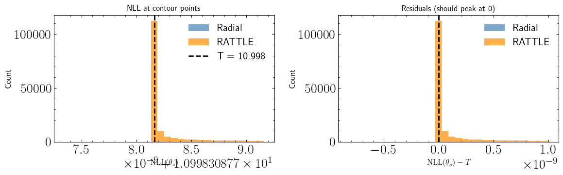
Max  |residual| : 1.00e-09
Mean |residual| : 7.31e-11

7 · Algorithm Walk-through

This section steps through each internal stage manually.

Stage 1 — Pre-whitening in signal-parameter space

find_contour evaluates the full \(4\times4\) Hessian of \(\log\mathcal{L}\) at \((\mu=1,\,\hat\theta_s)\), then extracts the \(3\times3\) signal-parameter block:

\[ G = -\bigl[\nabla^2\log\mathcal{L}\bigr]_{\text{signal indices}} \bigg|_{(\mu=1,\,\hat\theta_s)}. \]

After Cholesky factorisation \(G = LL^T\), the whitened coordinate \(\varphi = L(\theta_s - \hat\theta_s)\) makes the contour approximately spherical in the 3-D signal space.

# ── Full Hessian at (mu=1, theta_mle_signal) ─────────────────────────────────
hessian_fn = stat_model.backend.get_hessian_logpdf_func()
theta_mle_full = np.concatenate([[1.0], mle])  # [mu=1, c0_hat, c1_hat, c2_hat]

H_full = np.array(hessian_fn(theta_mle_full), dtype=float)  # 4×4
print("Full 4×4 Hessian of logpdf at (mu=1, θ̂s):")
print(np.round(H_full, 4))
print()

# ── Extract the 3×3 signal-parameter block ───────────────────────────────────
ix = np.ix_(signal_indices, signal_indices)
H_signal = H_full[ix]  # 3×3 block
G_signal = -H_signal  # Fisher information for signal params

print("3×3 signal-parameter block G = -H_signal:")
print(np.round(G_signal, 4))
print()

eigvals = np.linalg.eigvalsh(G_signal)
print(f"Eigenvalues of G: {eigvals.round(4)}")
print("(Large spread → strongly anisotropic → whitening is important)")

Full 4×4 Hessian of logpdf at (mu=1, θ̂s):
[[-2.0413  1.8607  0.9961  2.3241]
 [ 1.8607 -1.7084 -0.9474 -2.0542]
 [ 0.9961 -0.9474 -0.6137 -0.9256]
 [ 2.3241 -2.0542 -0.9256 -2.9886]]

3×3 signal-parameter block G = -H_signal:
[[1.7084 0.9474 2.0542]
 [0.9474 0.6137 0.9256]
 [2.0542 0.9256 2.9886]]

Eigenvalues of G: [2.0000e-04 4.1090e-01 4.8997e+00]
(Large spread → strongly anisotropic → whitening is important)

# ── Cholesky factorisation ─────────────────────────────────────────────────────
reg = 1e-8
w, V = np.linalg.eigh(G_signal)
w_reg = np.maximum(w, reg)
G_reg = (V * w_reg) @ V.T
L = np.linalg.cholesky(G_reg)

print("Cholesky factor L  (3×3):")
print(np.round(L, 4))
print()
print(f"Approx. whitened-space contour radius √Δ = {np.sqrt(delta):.4f}")
print("Radial search starts with this as the initial bracket radius.")

Cholesky factor L  (3×3):
[[ 1.3071  0.      0.    ]
 [ 0.7248  0.2972  0.    ]
 [ 1.5716 -0.7185  0.0478]]

Approx. whitened-space contour radius √Δ = 2.7955
Radial search starts with this as the initial bracket radius.

Stage 2 — Radial Search

For each random unit vector \(\hat{e}\) on \(S^2\), the algorithm solves

\[ f(r) = \mathrm{NLL}\!\bigl(\hat\theta_s + L^{-T}(r\hat{e})\bigr) - T = 0 \]

via Brent’s method. Note that the NLL here is always evaluated with \(\mu=1\):

\[ \mathrm{NLL}(\theta_s) = -\log\mathcal{L}\bigl(\mu{=}1,\,\theta_s\bigr). \]

from scipy.optimize import root_scalar

L_inv_T = np.linalg.solve(L, np.eye(k)).T  # L^{-T}

rng_demo = np.random.default_rng(7)
z = rng_demo.standard_normal(k)
e = z / np.linalg.norm(z)  # random unit vector on S²


def f(r):
    theta_s = mle + L_inv_T @ (r * e)
    return nll_fixed(theta_s) - result.threshold


r_vals = np.linspace(0.01, 6.0, 200)
f_vals = np.array([f(r) for r in r_vals])

r_hi = np.sqrt(delta)
while f(r_hi) <= 0 and r_hi < 30:
    r_hi *= 2
sol = root_scalar(f, bracket=[1e-8, r_hi], method="brentq", xtol=1e-12)
r_star = sol.root
theta_star = mle + L_inv_T @ (r_star * e)

fig, ax = plt.subplots(figsize=(8, 4))
ax.plot(r_vals, f_vals, color="steelblue", lw=2)
ax.axhline(0, color="k", lw=0.8)
ax.axvline(r_star, color="tomato", ls="--", lw=2, label=rf"$r^*$ = {r_star:.3f}")
ax.scatter([r_star], [0], color="tomato", s=80, zorder=5)
ax.set_xlabel(r"$r$  (whitened-space radius)", fontsize=12)
ax.set_ylabel(r"$f(r) = \mathrm{NLL}(\hat\theta_s + L^{-T}r\hat{e}) - T$", fontsize=11)
ax.set_title(r"Radial profile along one random direction ($\mu=1$ fixed)", fontsize=12)
ax.legend(fontsize=11)
plt.tight_layout()
plt.show()

print(f"Root r*      = {r_star:.4f}")
print(f"NLL(θ*)      = {nll_fixed(theta_star):.6f}")
print(f"Threshold T  = {result.threshold:.6f}")
print(f"Residual     = {abs(nll_fixed(theta_star) - result.threshold):.2e}")

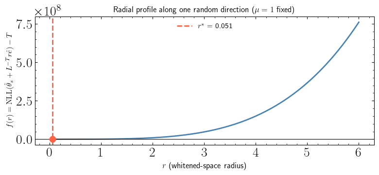
Root r*      = 0.0507
NLL(θ*)      = 10.998309
Threshold T  = 10.998309
Residual     = 9.91e-13

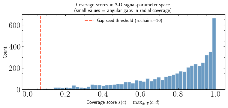
Stage 3 — Gap Detection

After the radial search, \(M \gg N\) candidate unit vectors \(c\) on \(S^2\) are sampled and scored by their maximum cosine similarity to the already-found directions:

\[ s(c) = \max_{d\in\mathcal{D}} \langle c, d \rangle. \]

The \(n_{\rm chains}\) candidates with the smallest \(s\) (largest angular gap) seed the RATTLE chains.

# ── Coverage scores over a large candidate set ───────────────────────────────
radial_pts = result.contour_points[result.from_radial]  # radial contour points

# Whitened directions corresponding to the radial contour points
phi_radial = (radial_pts - mle) @ L.T
dirs_radial = phi_radial / np.linalg.norm(phi_radial, axis=1, keepdims=True)

rng_gap = np.random.default_rng(99)
M = 5000
Z = rng_gap.standard_normal((M, k))
cands = Z / np.linalg.norm(Z, axis=1, keepdims=True)
cos_sim = cands @ dirs_radial.T
coverage = np.max(cos_sim, axis=1)

n_chains = 10
gap_threshold = np.sort(coverage)[n_chains]

fig, ax = plt.subplots(figsize=(8, 4))
ax.hist(coverage, bins=50, color="steelblue", alpha=0.8, edgecolor="white")
ax.axvline(
    gap_threshold,
    color="tomato",
    ls="--",
    lw=2,
    label=f"Gap-seed threshold (n_chains={n_chains})",
)
ax.set_xlabel(
    r"Coverage score $s(c) = \max_{d\in\mathcal{D}}\langle c,d\rangle$", fontsize=12
)
ax.set_ylabel("Count", fontsize=12)
ax.set_title(
    "Coverage scores in 3-D signal-parameter space\n"
    "(small values = angular gaps in radial coverage)",
    fontsize=12,
)
ax.legend(fontsize=11)
plt.tight_layout()
plt.show()

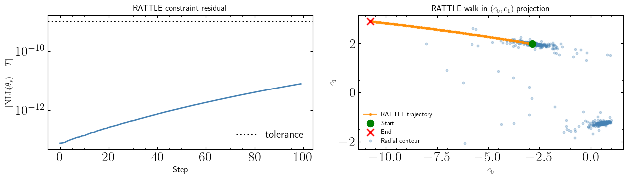
Stage 4 — Constrained RATTLE HMC

The RATTLE algorithm walks along the constraint surface \(C(\theta_s) = \mathrm{NLL}(\theta_s) - T = 0\) using gradient information. The NLL gradient is computed by autograd, which differentiates through the anp.concatenate([..., [1.0], ...]) insertion used to fix \(\mu=1\):

\[ \nabla_{\theta_s}\mathrm{NLL}(\theta_s) = \frac{\partial}{\partial\theta_s} \bigl[-\log\mathcal{L}(\mu{=}1,\theta_s)\bigr]. \]

One RATTLE leapfrog step (step size \(\varepsilon\)):

\[ p_{1/2} = p_0 - \tfrac{\varepsilon}{2}\nabla\mathrm{NLL}(\theta_0), \quad \theta' = \theta_0 + \varepsilon\,p_{1/2}, \]

\[ \theta_1 = \theta' - \frac{\mathrm{NLL}(\theta')-T}{|\nabla\mathrm{NLL}(\theta')|^2} \nabla\mathrm{NLL}(\theta'), \quad p_1 = \Bigl(p_{1/2} - \tfrac{\varepsilon}{2}\nabla\mathrm{NLL}(\theta_1)\Bigr)_{\perp \nabla\mathrm{NLL}(\theta_1)}. \]

import autograd
import autograd.numpy as anp

# ── Build autograd-differentiable NLL with mu=1 fixed ────────────────────────
logpdf_ag = stat_model.backend.get_logpdf_func()


def _nll_auto(signal_pars):
    """NLL(c0,c1,c2) with mu=1 inserted at poi_index=0; autograd-traced."""
    full_pars = anp.concatenate([anp.array([1.0]), signal_pars])
    return -logpdf_ag(full_pars)


_grad_auto = autograd.grad(_nll_auto)


def grad_nll(signal_pars):
    return np.array(_grad_auto(np.asarray(signal_pars, dtype=float)), dtype=float)


# ── Short RATTLE walk from a radial contour point ────────────────────────────
start = result.contour_points[0].copy()

# Project start onto constraint surface (handle tiny numerical drift)
theta_walk = start.copy()
for _ in range(50):
    res_val = nll_fixed(theta_walk) - result.threshold
    if abs(res_val) < 1e-9:
        break
    g = grad_nll(theta_walk)
    theta_walk -= (res_val / np.dot(g, g)) * g

# Initial tangent-space momentum
rng_walk = np.random.default_rng(1234)
g0 = grad_nll(theta_walk)
raw_p = rng_walk.standard_normal(k)
p_walk = raw_p - (np.dot(raw_p, g0) / np.dot(g0, g0)) * g0

eps = 0.05
trajectory = [theta_walk.copy()]
resid_track = []

for step in range(100):
    g = grad_nll(theta_walk)
    p_half = p_walk - (eps / 2) * g
    theta_prime = theta_walk + eps * p_half
    # SHAKE: Newton projection onto NLL = T
    for _ in range(100):
        rv = nll_fixed(theta_prime) - result.threshold
        if abs(rv) < 1e-9:
            break
        gp = grad_nll(theta_prime)
        theta_prime -= (rv / np.dot(gp, gp)) * gp
    g1 = grad_nll(theta_prime)
    p_prime = p_half - (eps / 2) * g1
    p_walk = p_prime - (np.dot(p_prime, g1) / np.dot(g1, g1)) * g1  # tangent proj.
    theta_walk = theta_prime
    trajectory.append(theta_walk.copy())
    resid_track.append(abs(nll_fixed(theta_walk) - result.threshold))

trajectory = np.array(trajectory)

# ── Plots ─────────────────────────────────────────────────────────────────────
fig, axes = plt.subplots(1, 2, figsize=(13, 4))

axes[0].semilogy(resid_track, color="steelblue", lw=2)
axes[0].axhline(1e-9, color="k", ls=":", label="tolerance")
axes[0].set_xlabel("Step", fontsize=12)
axes[0].set_ylabel(r"$|\mathrm{NLL}(\theta_s) - T|$", fontsize=12)
axes[0].set_title("RATTLE constraint residual", fontsize=12)
axes[0].legend()

axes[1].plot(
    trajectory[:, 0],
    trajectory[:, 1],
    "o-",
    color="darkorange",
    ms=3,
    lw=1.5,
    alpha=0.8,
    label="RATTLE trajectory",
)
axes[1].scatter(
    trajectory[0, 0], trajectory[0, 1], s=100, color="green", zorder=5, label="Start"
)
axes[1].scatter(
    trajectory[-1, 0],
    trajectory[-1, 1],
    s=100,
    color="red",
    marker="x",
    zorder=5,
    label="End",
)
axes[1].scatter(
    radial_pts[:, 0],
    radial_pts[:, 1],
    s=10,
    alpha=0.3,
    color="steelblue",
    label="Radial contour",
)
axes[1].set_xlabel(r"$c_0$", fontsize=12)
axes[1].set_ylabel(r"$c_1$", fontsize=12)
axes[1].set_title(r"RATTLE walk in $(c_0, c_1)$ projection", fontsize=12)
axes[1].legend(fontsize=9)

plt.tight_layout()
plt.show()

Summary

In this notebook we have:

1. Built a statistical model with four backend parameters \([\mu, c_0, c_1, c_2]\) using MultivariateNormal with n_signal_parameters=3.

2. Fixed \(\mu=1\) throughout the analysis. find_contour uses cfg.poi_index to identify and exclude the signal strength from the contour search, then inserts \(\mu=1\) at every NLL evaluation via autograd.numpy.concatenate — keeping the function autograd-differentiable.

3. Found the MLE \((\hat c_0, \hat c_1, \hat c_2)\) by passing fixed_poi_value=1.0 to the spey optimizer, which holds \(\mu\) fixed while minimising over the signal-shape parameters.

4. Mapped the 95% CL contour — the 2-D surface in the 3-D \((c_0, c_1, c_2)\) space where \(\chi^2_{k=3}(\theta_s) = \Delta_{0.95} \approx 7.81\) — using:

   • Radial search in pre-whitened signal-parameter space, and

   • Constrained RATTLE HMC to fill angular gaps.

5. Visualised the result as pairwise 2-D projections and a 3-D scatter plot.

Further reading

• Wilks (1938), Ann. Math. Stat.

• Andersen (1983), J. Comput. Phys. — RATTLE algorithm

• spey.multiparameter.contour module — full mathematical derivation in module docstring