Quick Start

Installation

spey is available at pypi , so it can be installed by running:

>>> pip install spey

Python >=3.8 is required. spey heavily relies on numpy, scipy and autograd which are all packaged during the installation with the necessary versions. Note that some versions may be restricted due to numeric stability and validation.

What is Spey?

Spey is a plug-in-based statistics tool designed to consolidate a wide range of likelihood prescriptions in a comprehensive platform. Spey empowers users to integrate different statistical models seamlessly and explore their properties through a unified interface by offering a flexible workspace. To ensure compatibility with existing and future statistical model prescriptions, Spey adopts a versatile plug-in system. This approach enables developers to propose and integrate their statistical model prescriptions, thereby expanding the capabilities and applicability of Spey.

First Steps

First, one needs to choose which backend to work with. By default, Spey is shipped with various types of likelihood prescriptions which can be checked via AvailableBackends() function

>>> import spey
>>> print(spey.AvailableBackends())
>>> # ['default_pdf.correlated_background',
>>> #  'default_pdf.effective_sigma',
>>> #  'default_pdf.third_moment_expansion',
>>> #  'default_pdf.uncorrelated_background']

For details on all the backends, see Plug-ins section.

Using 'default_pdf.uncorrelated_background' one can simply create single or multi-bin statistical models:

>>> pdf_wrapper = spey.get_backend('default_pdf.uncorrelated_background')

>>> data = [1]
>>> signal_yields = [0.5]
>>> background_yields = [2.0]
>>> background_unc = [1.1]

>>> stat_model = pdf_wrapper(
...     signal_yields=signal_yields,
...     background_yields=background_yields,
...     data=data,
...     absolute_uncertainties=background_unc,
...     analysis="single_bin",
...     xsection=0.123,
... )

where data indicates the observed events, signal_yields and background_yields represents yields for signal and background samples and background_unc shows the absolute uncertainties on the background events, i.e. \(2.0\pm1.1\) in this particular case. Note that we also introduced analysis and xsection information which are optional where the analysis indicates an unique identifier for the statistical model, and xsection is the cross-section value of the signal, which is only used for the computation of the excluded cross-section value.

During the computation of any probability distribution, Spey relies on the so-called “expectation type”. This can be set via ExpectationType, which includes three different expectation modes.

• observed: Indicates that the computation of the log-probability will be achieved by fitting the statistical model on the experimental data. For the exclusion limit computation, this will tell the package to compute observed \(1-CL_s\) values. observed has been set as default throughout the package.

• aposteriori: This command will result in the same log-probability computation as observed. However, the expected exclusion limit will be computed by centralising the statistical model on the background and checking \(\pm1\sigma\) and \(\pm2\sigma\) fluctuations.

• apriori: Indicates that the observation has never taken place and the theoretical SM computation is the absolute truth. Thus, it replaces observed values in the statistical model with the background values and computes the log-probability accordingly. Similar to aposteriori Exclusion limit computation will return expected limits.

To compute the observed exclusion limit for the above example, one can type

>>> for expectation in spey.ExpectationType:
>>>     print(f"1-CLs ({expectation}): {stat_model.exclusion_confidence_level(expected=expectation)}")
>>> # 1-CLs (apriori): [0.49026742260475775, 0.3571003642744075, 0.21302512037071475, 0.1756147641077802, 0.1756147641077802]
>>> # 1-CLs (aposteriori): [0.6959976874809755, 0.5466491036450178, 0.3556261845401908, 0.2623335168616665, 0.2623335168616665]
>>> # 1-CLs (observed): [0.40145846656558726]

Note that apriori and aposteriori expectation types resulted in a list of 5 elements which indicates \(-2\sigma,\ -1\sigma,\ 0,\ +1\sigma,\ +2\sigma\) standard deviations from the background hypothesis. observed, on the other hand, resulted in a single value, which is the observed exclusion limit. Notice that the bounds on aposteriori are slightly more potent than apriori; this is due to the data value has been replaced with background yields, which are larger than the observations. apriori is mainly used in theory collaborations to estimate the difference from the Standard Model rather than the experimental observations.

Note

For details on exclusion limit and upper limit computations, see ref. [1].

One can play the same game using the same backend for multi-bin histograms as follows;

>>> pdf_wrapper = spey.get_backend('default_pdf.uncorrelated_background')

>>> data = [36, 33]
>>> signal_yields = [12.0, 15.0]
>>> background_yields = [50.0,48.0]
>>> background_unc = [12.0,16.0]

>>> stat_model = pdf_wrapper(
...     signal_yields=signal_yields,
...     background_yields=background_yields,
...     data=data,
...     absolute_uncertainties=background_unc,
...     analysis="multi_bin",
...     xsection=0.123,
... )

Note that our statistical model still represents individual bins of the histograms independently however, it sums up the log-likelihood of each bin. Hence, all bins are completely uncorrelated from each other. Computing the exclusion limits for each ExpectationType will yield

>>> for expectation in spey.ExpectationType:
>>>     print(f"1-CLs ({expectation}): {stat_model.exclusion_confidence_level(expected=expectation)}")
>>> # 1-CLs (apriori): [0.971099302028661, 0.9151646569018123, 0.7747509673901924, 0.5058089246145081, 0.4365406649302913]
>>> # 1-CLs (aposteriori): [0.9989818194986659, 0.9933308419577298, 0.9618669253593897, 0.8317680908087413, 0.5183060229282643]
>>> # 1-CLs (observed): [0.9701795436411219]

It is also possible to compute \(1-CL_s\) value with respect to the parameter of interest, \(\mu\). This can be achieved by including a value for poi_test argument

>>> import matplotlib.pyplot as plt
>>> import numpy as np

>>> poi = np.linspace(0,10,20)
>>> poiUL = np.array([stat_model.exclusion_confidence_level(poi_test=p, expected=spey.ExpectationType.aposteriori) for p in poi])
>>> plt.plot(poi, poiUL[:,2], color="tab:red")
>>> plt.fill_between(poi, poiUL[:,1], poiUL[:,3], alpha=0.8, color="green", lw=0)
>>> plt.fill_between(poi, poiUL[:,0], poiUL[:,4], alpha=0.5, color="yellow", lw=0)
>>> plt.plot([0,10], [.95,.95], color="k", ls="dashed")
>>> plt.xlabel(r"${\rm signal\ strength}\ (\mu)$")
>>> plt.ylabel("$1-CL_s$")
>>> plt.xlim([0,10])
>>> plt.ylim([0.6,1.01])
>>> plt.text(0.5,0.96, r"$95\%\ {\rm CL}$")
>>> plt.show()

Here in the first line, we extract \(1-CL_s\) values per POI for aposteriori expectation type, and we plot specific standard deviations, which provides the following plot:

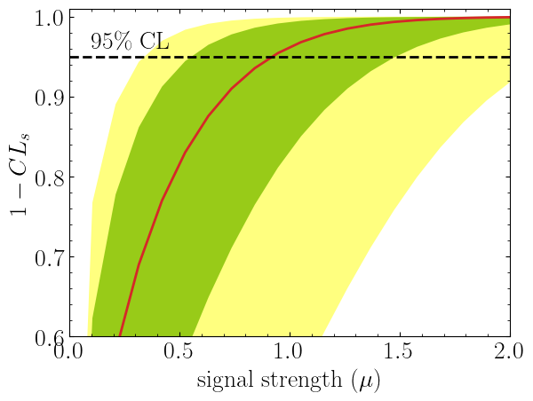
The excluded value of POI can also be retrieved by poi_upper_limit() function

>>> print("POI UL: %.3f" % stat_model.poi_upper_limit(expected=spey.ExpectationType.aposteriori))
>>> # POI UL:  0.920

which is the exact point where the red curve and black dashed line meet. The upper limit for the \(\pm1\sigma\) or \(\pm2\sigma\) bands can be extracted by setting expected_pvalue to "1sigma" or "2sigma" respectively, e.g.

>>> stat_model.poi_upper_limit(expected=spey.ExpectationType.aposteriori, expected_pvalue="1sigma")
>>> # [0.5507713378348318, 0.9195052042538805, 1.4812721449679866]

At a lower level, one can extract the likelihood information for the statistical model by calling likelihood() and maximize_likelihood() functions. By default, these will return negative log-likelihood values, but this can be changed via return_nll=False argument.

>>> muhat_obs, maxllhd_obs = stat_model.maximize_likelihood(return_nll=False, )
>>> muhat_apri, maxllhd_apri = stat_model.maximize_likelihood(return_nll=False, expected=spey.ExpectationType.apriori)

>>> poi = np.linspace(-3,4,60)

>>> llhd_obs = np.array([stat_model.likelihood(p, return_nll=False) for p in poi])
>>> llhd_apri = np.array([stat_model.likelihood(p, expected=spey.ExpectationType.apriori, return_nll=False) for p in poi])

Here in first two lines, we extracted maximum likelihood and the POI value that maximises the likelihood for two different expectation type. In the following, we computed likelihood distribution for various POI values, which then can be plotted as follows

>>> plt.plot(poi, llhd_obs/maxllhd_obs, label=r"${\rm observed\ or\ aposteriori}$")
>>> plt.plot(poi, llhd_apri/maxllhd_apri, label=r"${\rm apriori}$")
>>> plt.scatter(muhat_obs, 1)
>>> plt.scatter(muhat_apri, 1)
>>> plt.legend(loc="upper right")
>>> plt.ylabel(r"$\mathcal{L}(\mu,\theta_\mu)/\mathcal{L}(\hat\mu,\hat\theta)$")
>>> plt.xlabel(r"${\rm signal\ strength}\ (\mu)$")
>>> plt.ylim([0,1.3])
>>> plt.xlim([-3,4])
>>> plt.show()

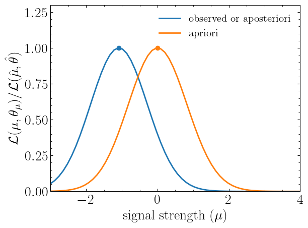
Notice the slight difference between likelihood distributions because of the use of different expectation types. The dots on the likelihood distribution represent the point where the likelihood is maximised. Since for an apriori likelihood distribution observed and background values are the same, the likelihood should peak at \(\mu=0\).