Introduction to Spey: A Unified Statistical Inference Framework#

Motivation#

The search for physics beyond the Standard Model at the LHC requires rigorous statistical inference on data from complex, multi-bin signal regions. Different experimental analyses provide background estimates in different forms — covariance matrices, asymmetric uncertainty envelopes, full likelihood models in pyhf format — and reinterpretation studies must handle all of these consistently.

Spey (arXiv:2307.06996) addresses this by providing a common API for statistical inference in high-energy physics. The core idea is a backend (or plugin) architecture: each backend encapsulates a specific likelihood prescription — a mathematical model for how the observed data were generated — and exposes it through a uniform interface. A user constructs a StatisticalModel object by choosing a backend and supplying the relevant inputs (signal yields, background yields, uncertainties, observed data). All subsequent operations — evaluating the likelihood, computing upper limits, exclusion confidence levels — are then called identically regardless of which backend was chosen.

This notebook demonstrates Spey’s capabilities using published data from the CMS-SUS-20-004 analysis. We will construct three different likelihood models for the same dataset and compare their predictions.

The imports above bring in the core spey package, numpy for array manipulation, matplotlib for plotting, and scipy for numerical routines. The version numbers are printed for reproducibility.

The Plugin Architecture#

Spey uses a plugin system where each registered backend implements a self-contained likelihood prescription. A backend is a Python package that follows a specific interface contract (see arXiv:2307.06996, Appendix A, for the specification). Once installed, backends register themselves under a namespaced key such as "default.correlated_background" or "pyhf".

The full list of currently installed backends is returned by spey.AvailableBackends():

spey.AvailableBackends()

['hs3',
 'default.correlated_background',
 'default.effective_sigma',
 'default.multivariate_normal',
 'default.normal',
 'default.poisson',
 'default.third_moment_expansion',
 'default.uncorrelated_background',
 'pyhf',
 'pyhf.simplify',
 'pyhf.uncorrelated_background']

Each backend carries citation metadata — author information, version, DOI, and arXiv identifiers — so that users can automatically generate proper references for the likelihood prescriptions they employ. This metadata is accessible via spey.get_backend_metadata(), and the corresponding BibTeX entries can be retrieved with spey.get_backend_bibtex(). As an example, let us inspect the metadata for the third moment expansion backend:

spey.get_backend_metadata("default.third_moment_expansion")

{'name': 'default.third_moment_expansion',
 'author': 'SpeysideHEP',
 'version': '0.2.7-b2',
 'spey_requires': '0.2.7-b2',
 'doi': ['10.1007/JHEP04(2019)064'],
 'arXiv': ['1809.05548'],
 'zenodo': []}

spey.get_backend_bibtex("default.third_moment_expansion")

{'inspire': ['    @article{Buckley:2018vdr,\n        author = "Buckley, Andy and Citron, Matthew and Fichet, Sylvain and Kraml, Sabine and Waltenberger, Wolfgang and Wardle, Nicholas",\n        title = "{The Simplified Likelihood Framework}",\n        eprint = "1809.05548",\n        archivePrefix = "arXiv",\n        primaryClass = "hep-ph",\n        doi = "10.1007/JHEP04(2019)064",\n        journal = "JHEP",\n        volume = "04",\n        pages = "064",\n        year = "2019"\n    }\n',
  '    @article{Buckley:2018vdr,\n        author = "Buckley, Andy and Citron, Matthew and Fichet, Sylvain and Kraml, Sabine and Waltenberger, Wolfgang and Wardle, Nicholas",\n        title = "{The Simplified Likelihood Framework}",\n        eprint = "1809.05548",\n        archivePrefix = "arXiv",\n        primaryClass = "hep-ph",\n        doi = "10.1007/JHEP04(2019)064",\n        journal = "JHEP",\n        volume = "04",\n        pages = "064",\n        year = "2019"\n    }\n'],
 'doi.org': [],
 'zenodo': []}

Custom backends implementing user-defined likelihood prescriptions can be developed following the plugin specification in arXiv:2307.06996 and the online documentation.

Statistical Framework#

Profile Likelihood Ratio Test Statistic#

Hypothesis testing in HEP is typically carried out using the profile likelihood ratio test statistic. Let \(\mu\) denote the signal strength parameter of interest (POI) and \(\boldsymbol{\theta}\) a vector of nuisance parameters encoding systematic uncertainties. The profile likelihood ratio is

\[ q_\mu = -2\ln\frac{\mathcal{L}(\mu, \hat{\hat{\boldsymbol{\theta}}}_\mu)}{\mathcal{L}(\hat{\mu}, \hat{\boldsymbol{\theta}})}, \]

where \((\hat{\mu}, \hat{\boldsymbol{\theta}})\) are the unconditional (global) maximum likelihood estimators, and \(\hat{\hat{\boldsymbol{\theta}}}_\mu\) are the nuisance parameters that maximise the likelihood at fixed \(\mu\) (the profiled nuisance parameters). By Wilks’ theorem, \(q_\mu\) is asymptotically distributed as \(\chi^2_1\) under the hypothesis \(\mu\), which enables \(p\)-value calculations without Monte Carlo simulations.

The CLs Method#

A naive \(p\)-value cut can result in spurious exclusions of signal hypotheses in regions where the experiment has little sensitivity (e.g., when the signal is very small and the data fluctuate downward). The CLs method (Read, 2002) guards against this by constructing the ratio

\[ \mathrm{CL}_s(\mu) = \frac{p_{s+b}(\mu)}{1 - p_b}, \]

where \(p_{s+b}(\mu)\) is the \(p\)-value of the observed data under the signal-plus-background hypothesis at strength \(\mu\), and \(p_b\) is the \(p\)-value under the background-only hypothesis. A signal hypothesis is excluded at 95% CL when \(\mathrm{CL}_s(\mu) < 0.05\), equivalently \(1 - \mathrm{CL}_s > 0.95\). The penalisation by \(1 - p_b\) suppresses exclusions in low-sensitivity regions.

Asimov Dataset#

An Asimov dataset (Cowan, Cranmer, Gross, Vitells, 2011) is a representative pseudo-dataset in which every observable is replaced by its expected value under a given hypothesis. In practice, the background-only Asimov dataset sets the observed counts equal to the expected background yields (after fitting the nuisance parameters). Using the Asimov dataset in place of real observations gives the expected (pre-fit) sensitivity of the analysis — the limit one would obtain on average in an ensemble of background-only experiments — without running computationally expensive toy experiments.

Experimental Data: CMS-SUS-20-004#

We use data from the CMS-SUS-20-004 analysis, which searches for electroweakino pair production

\[ pp \to \tilde{\chi}^0_3\tilde{\chi}^0_2 \to HH\tilde{\chi}^0_1\tilde{\chi}^0_1 \]

in final states with two Higgs bosons and missing transverse energy. The specific mass point used here is \(m_{\tilde{\chi}^0_1} = 50\,\mathrm{GeV}\) and \(m_{\tilde{\chi}^0_{3,2}} = 300\,\mathrm{GeV}\). The analysis employs a multi-bin signal region, providing sufficient statistical power to test the simplified likelihood approximations described below.

The data are publicly available at Zenodo (doi:10.5281/zenodo.10008261) and contain the following arrays:

Array	Description
`observations`	Observed event counts in each signal region bin
`background_yields`	Expected background yields per bin from Monte Carlo simulation
`background_uncertainty`	Symmetric per-bin background uncertainties (\(\sigma_b^i\))
`covariance_matrix`	Full bin-by-bin covariance matrix \(\Sigma_{ij}\) encoding inter-bin correlations
`third_moments`	Third central moments \(m^{(3)}_i\) of the background distribution per bin
`upper_unc_envelope`	Upper asymmetric uncertainty envelope \(\sigma^+_i\) per bin
`lower_unc_envelope`	Lower asymmetric uncertainty envelope \(\sigma^-_i\) per bin
`signal_yields`	Predicted signal event counts per bin for the chosen mass point

Simplified Likelihood: Correlated Background Model#

The most widely-used approximation for LHC reinterpretation studies is the simplified likelihood (CMS-NOTE-2017-001). CMS and ATLAS routinely publish background yields together with a covariance matrix that encodes systematic and statistical correlations between bins. The likelihood is

\[ \mathcal{L}(\mu, \boldsymbol{\theta}) = \prod_{i \in \mathrm{bins}} \mathrm{Poiss}\!\left(n^i \,\Big|\, \mu\, n_s^i + n_b^i + \sum_j \theta^j L^{ij}\right) \cdot \prod_{j \in \mathrm{nui}} \mathcal{N}(\theta^j \,|\, 0, 1), \]

where \(L\) is the lower-triangular Cholesky factor of the covariance matrix, \(\Sigma = LL^T\). The nuisance parameters \(\boldsymbol{\theta}\) are standard-normal auxiliary measurements; integrating them out recovers the correct inter-bin covariance structure. An equivalent, more transparent form is

\[ \mathcal{L}(\mu, \boldsymbol{\theta}) = \prod_{i} \mathrm{Poiss}\!\left(n^i \,\Big|\, \mu\, n_s^i + n_b^i + \theta^i\sigma_b^i\right) \cdot \mathcal{N}(\boldsymbol{\theta} \,|\, \boldsymbol{0}, \rho), \]

where \(\rho_{ij} = \Sigma_{ij}/(\sigma_b^i \sigma_b^j)\) is the bin-by-bin correlation matrix and \(\sigma_b^i = \sqrt{\Sigma_{ii}}\) are the marginal background uncertainties. Here \(n^i\), \(n_s^i\), and \(n_b^i\) denote the observed counts, signal yields, and background yields in bin \(i\), respectively, \(\mu\) is the signal strength (POI), and \(\boldsymbol{\theta}\) are the nuisance parameters.

In Spey this prescription is identified as "default.correlated_background". We first retrieve the backend wrapper with spey.get_backend() and then construct the StatisticalModel object:

pdf_wrapper = spey.get_backend("default.correlated_background")

corr_background_model = pdf_wrapper(
    signal_yields=signal_yields,
    background_yields=background_yields,
    data=observations,
    covariance_matrix=covariance_matrix,
    analysis="cms-sus-20-004-SL",
)
print(corr_background_model)

StatisticalModel(analysis='cms-sus-20-004-SL', backend=default.correlated_background, calculators=['toy', 'asymptotic', 'chi_square'])

Every likelihood prescription in Spey is represented by the StatisticalModel class. This backend-agnostic wrapper means that all likelihood prescriptions share an identical interface: once the model object is constructed, the statistical analysis proceeds identically regardless of which backend underlies it.

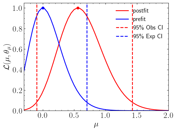
Profile Likelihood and Confidence Intervals#

With the model built, we can evaluate the profile likelihood and locate the maximum likelihood estimate:

likelihood(mu, return_nll=False) evaluates the profile likelihood \(\mathcal{L}(\mu, \hat{\hat{\boldsymbol{\theta}}}_\mu)\), where the nuisance parameters are profiled (maximised) at each fixed value of \(\mu\). Setting return_nll=False returns the likelihood itself rather than the negative log-likelihood.
maximize_likelihood() finds the global MLE \((\hat{\mu}, \hat{\boldsymbol{\theta}})\) and returns the pair \((\hat{\mu},\, -\ln\mathcal{L}(\hat{\mu}, \hat{\boldsymbol{\theta}}))\).
expected=spey.ExpectationType.apriori replaces the observed data with the background-only Asimov dataset, giving the pre-fit (expected) likelihood scan that represents the analysis sensitivity independent of the actual observation. The default behaviour (without this flag, or with aposteriori) uses the actual observed data.
chi2_test() applies Wilks’ theorem: under the asymptotic approximation \(-2(\ln\mathcal{L}(\mu, \hat{\hat{\boldsymbol{\theta}}}_\mu) - \ln\mathcal{L}(\hat{\mu}, \hat{\boldsymbol{\theta}})) \sim \chi^2_1\), so the 95% confidence interval on \(\mu\) is the set of values for which this quantity is less than \(\chi^2_1(0.95) \approx 3.84\).

Note

By default likelihood and maximize_likelihood return the negative log-likelihood. To obtain the likelihood itself, set return_nll=False.

Attention

The POI scan starts from \(\mu = -0.3\) because at more negative values the expected Poisson rate \(\mu n_s^i + n_b^i\) would become negative in some bins, rendering the Poisson likelihood undefined. The minimum allowed POI can be queried via corr_background_model.backend.config().minimum_poi.

poi = np.linspace(-0.3, 2, 50)

llhd_postfit = [corr_background_model.likelihood(p, return_nll=False) for p in poi]
muhat_postfit, max_llhd_postfit = corr_background_model.maximize_likelihood(
    return_nll=False
)

llhd_prefit = [
    corr_background_model.likelihood(
        p, expected=spey.ExpectationType.apriori, return_nll=False
    )
    for p in poi
]
muhat_prefit, max_llhd_prefit = corr_background_model.maximize_likelihood(
    expected=spey.ExpectationType.apriori, return_nll=False
)

The 95% confidence interval on \(\mu\) derived from the chi-square test is shown as vertical dashed lines in the plot below:

obs_lo, obs_up = corr_background_model.chi2_test()
exp_lo, exp_up = corr_background_model.chi2_test(expected=spey.ExpectationType.apriori)

Upper Limits and CLs Exclusion#

Beyond confidence intervals, the main outputs for LHC reinterpretation are:

poi_upper_limit() finds the value \(\mu^{95}\) such that \(\mathrm{CL}_s(\mu^{95}) = 0.05\), i.e. the 95% CL upper limit on the signal strength. The confidence level can be changed via the confidence_level argument.
exclusion_confidence_level(poi_test=1.0) returns \(1 - \mathrm{CL}_s(\mu_\mathrm{test})\) for a given test signal strength (default \(\mu_\mathrm{test} = 1\)). Values above 0.95 indicate exclusion of the signal hypothesis at 95% CL.
expected=spey.ExpectationType.aposteriori computes the post-fit expected limit: the expected limit conditioned on the observed data, obtained by generating pseudo-experiments around the observed yield. This accounts for any upward or downward fluctuation in the data.
expected=spey.ExpectationType.apriori computes the pre-fit expected limit using the background-only Asimov dataset, independent of the actual observation.
expected_pvalue="1sigma" additionally returns the \(\pm 1\sigma\) uncertainty band on the expected limit, yielding a 3-tuple \([\mu^{-1\sigma},\, \mu^\mathrm{central},\, \mu^{+1\sigma}]\).
generate_asimov_data() returns the Asimov dataset — the expected event yields under the background-only hypothesis after fitting the nuisance parameters to their central values.

Let us first inspect the likelihood maximum and the Asimov dataset:

print(corr_background_model.maximize_likelihood())
print(corr_background_model.maximize_asimov_likelihood())
print(corr_background_model.generate_asimov_data())

(0.5593035620586441, 65.89866979012393)
(0.06572762944448773, 53.623166396006525)
[1.48714607e+02 9.12960774e+01 1.27426703e+01 2.76593162e+00
37834420e+01 3.28223804e+01 3.17408580e+00 1.48416222e-08
77525461e+00 2.26729359e+00 2.51993080e-01 9.54610346e-09
51752825e+00 1.54387041e+00 7.47061388e-01 7.24000104e-01
67057680e+01 7.21012058e+00 1.47068621e+00 4.00553317e+00
74932825e-01 8.58054701e-02 0.00000000e+00 0.00000000e+00
00000000e+00 0.00000000e+00 0.00000000e+00 0.00000000e+00
00000000e+00 0.00000000e+00 0.00000000e+00 0.00000000e+00
00000000e+00 0.00000000e+00 0.00000000e+00 0.00000000e+00
00000000e+00 0.00000000e+00 0.00000000e+00 0.00000000e+00
00000000e+00 0.00000000e+00 0.00000000e+00 0.00000000e+00]

print(
    f"Observed upper limit on µ at 95% CL: {corr_background_model.poi_upper_limit():.5f}"
)

expected_pval = corr_background_model.poi_upper_limit(
    expected=spey.ExpectationType.aposteriori, expected_pvalue="1sigma"
)
muUL_apost = expected_pval[1]
print(
    "Expected upper limit on µ with ± 1σ at 95% CL: "
    + ",".join([f"{x:.3f}" for x in expected_pval])
)

Observed upper limit on µ at 95% CL: 1.19563
Expected upper limit on µ with ± 1σ at 95% CL: 0.564,0.761,1.058

print(
    f"Observed upper limit on µ at 68% CL: {corr_background_model.poi_upper_limit(confidence_level=0.68):.5f}"
)

Observed upper limit on µ at 68% CL: 0.75204

We can also compute \(\mathrm{CL}_s(\mu)\) explicitly over a grid of signal strength values and plot the CLs scan to visualise where the 95% exclusion threshold is crossed:

poi = np.linspace(0, 1.5, 20)
poiUL = np.array(
    [
        corr_background_model.exclusion_confidence_level(
            poi_test=p, expected=spey.ExpectationType.aposteriori
        )
        for p in poi
    ]
)

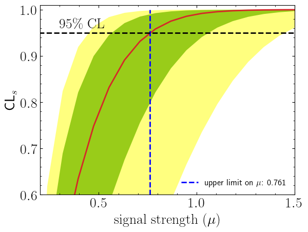
../_images/bc21ea46d4a66ec8e91a2c73129bb2f66c1d97dc5906babf6a962c18c58a94f9.png

print(
    f"Observed exclusion confidence level, CLs: {corr_background_model.exclusion_confidence_level()[0]:.5f}"
)

Observed exclusion confidence level, CLs: 0.87389

exp_cls = corr_background_model.exclusion_confidence_level(
    expected=spey.ExpectationType.aposteriori
)
print(
    f"Expected exclusion confidence level, CLs ± 1σ: {exp_cls[2]:.4f} - {exp_cls[2]-exp_cls[3]:.4f} + {exp_cls[1]-exp_cls[2]:.4f}"
)

Expected exclusion confidence level, CLs ± 1σ: 0.9902 - 0.0578 + 0.0088

More details on exclusion limit computation, including the treatment of one-sided and two-sided test statistics, can be found in the dedicated documentation section.

Third Moment Expansion#

The simplified likelihood assumes that background uncertainties are symmetric and Gaussian. In practice, background distributions — especially those arising from MC re-weighting or extrapolation from control regions — can be substantially skewed. The third moment expansion of Buckley, Citron, Fichet, Kraml, Waltenberger, and Wardle (arXiv:1809.05548, JHEP 2019) extends the simplified likelihood to capture this asymmetry.

The key idea is to expand the Poisson rate as a quadratic function of the nuisance parameter \(\theta_i\):

\[ \lambda^i(\theta_i) = \mu\, n_s^i + \bar{n}_b^i + B_i\theta_i + S_i\theta_i^2, \]

where the three coefficients are determined by matching the first three moments of the background distribution:

\(\bar{n}_b^i\): central background value,
\(B_i = \sqrt{\sigma_b^{i\,2} - 2S_i^2}\): effective standard deviation,
\(S_i = m_i^{(3)}/6\): skewness coefficient, where \(m_i^{(3)}\) is the third central moment of the background.

The full likelihood is:

\[ \mathcal{L}(\mu, \boldsymbol{\theta}) = \prod_{i\in\mathrm{bins}}\mathrm{Poiss}\!\left(n^i \,\Big|\, \mu\, n_s^i + \bar{n}_b^i + B_i\theta_i + S_i\theta_i^2\right) \cdot \prod_{j}\mathcal{N}(\theta^j \,|\, 0, \bar{\rho}), \]

where \(\bar{\rho}\) is the bin-by-bin correlation matrix. When the third central moments \(m_i^{(3)}\) are not published directly but asymmetric uncertainty envelopes \(\sigma^\pm_i\) are available, Spey can approximate them using the bifurcated Gaussian assumption:

\[ m^{(3)} = \frac{2}{\sigma^+ + \sigma^-} \left[ \sigma^-\int_{-\infty}^0 x^3\mathcal{N}(x|0,\sigma^-)\,dx + \sigma^+ \int_0^{\infty} x^3\mathcal{N}(x|0,\sigma^+)\,dx \right], \]

via the compute_third_moments function. When the experiment provides explicit third moments (as in this dataset), those should always be used directly.

In Spey this prescription is "default.third_moment_expansion":

Question:

Experimental collaboration provided asymmetric uncertainties but not third moments, can spey compute third moments?

Answer: Yes! one can use compute_third_moments function which computes third moments using Bifurcated Gaussian

\[ m^{(3)} = \frac{2}{\sigma^+ + \sigma^-} \left[ \sigma^-\int_{-\infty}^0 x^3\mathcal{N}(x|0,\sigma^-)dx + \sigma^+ \int_0^{\infty} x^3\mathcal{N}(x|0,\sigma^+)dx \right] \]

But this is an assumption, if collaboration provides exact third moments, please always use those.

pdf_wrapper = spey.get_backend("default.third_moment_expansion")
third_mom_expansion_model = pdf_wrapper(
    signal_yields=signal_yields,
    background_yields=background_yields,
    data=observations,
    covariance_matrix=covariance_matrix,
    third_moment=third_moments,
    analysis="cms-sus-20-004-TM",
)
print(third_mom_expansion_model)

StatisticalModel(analysis='cms-sus-20-004-TM', backend=default.third_moment_expansion, calculators=['toy', 'asymptotic', 'chi_square'])

print(f"Observed upper limit on µ: {third_mom_expansion_model.poi_upper_limit():.5f}")
print(
    f"Expected upper limit on µ: {third_mom_expansion_model.poi_upper_limit(expected=spey.ExpectationType.aposteriori):.5f}"
)
print(
    f"Observed exclusion confidence level, CLs: {third_mom_expansion_model.exclusion_confidence_level()[0]:.5f}"
)

Observed upper limit on µ: 1.17413
Expected upper limit on µ: 0.81700
Observed exclusion confidence level, CLs: 0.88502

Effective Sigma#

A complementary approach to handling asymmetric uncertainties is the effective sigma (or Variable Gaussian) method of Barlow (arXiv:physics/0406120). Rather than expanding the Poisson rate as a polynomial in \(\theta\), it makes the uncertainty itself a smooth function of the nuisance parameter:

\[ \sigma_{\rm eff}^i(\theta^i) = \sqrt{\sigma^+_i\sigma^-_i + (\sigma^+_i - \sigma^-_i)\,\theta^i}, \]

which interpolates between \(\sigma^-_i\) for \(\theta^i \ll 0\) and \(\sigma^+_i\) for \(\theta^i \gg 0\), with \(\sigma_{\rm eff}^i(0) = \sqrt{\sigma^+_i\sigma^-_i}\) at the central value. The full likelihood is:

\[ \mathcal{L}(\mu, \boldsymbol{\theta}) = \prod_{i\in\mathrm{bins}}\mathrm{Poiss}\!\left(n^i \,\Big|\, \mu\, n_s^i + n_b^i + \theta^i\sigma_{\rm eff}^i(\theta^i)\right) \cdot \mathcal{N}(\boldsymbol{\theta} \,|\, \boldsymbol{0}, \rho), \]

where \(\rho\) is the bin-by-bin correlation matrix. Note that this backend takes a correlation matrix rather than a covariance matrix; the conversion is performed with spey.helper_functions.covariance_to_correlation. In Spey this prescription is "default.effective_sigma":

pdf_wrapper = spey.get_backend("default.effective_sigma")
effective_sigma_model = pdf_wrapper(
    signal_yields=signal_yields,
    background_yields=background_yields,
    data=observations,
    correlation_matrix=covariance_to_correlation(covariance_matrix),
    absolute_uncertainty_envelops=[
        (up, dn) for up, dn in zip(upper_unc_envelope, lower_unc_envelope)
    ],
    analysis="cms-sus-20-004-ES",
)
print(effective_sigma_model)

StatisticalModel(analysis='cms-sus-20-004-ES', backend=default.effective_sigma, calculators=['toy', 'asymptotic', 'chi_square'])

print(f"Observed upper limit on µ: {effective_sigma_model.poi_upper_limit():.5f}")
print(
    f"Expected upper limit on µ: {effective_sigma_model.poi_upper_limit(expected=spey.ExpectationType.aposteriori):.5f}"
)
print(
    f"Observed exclusion confidence level, CLs: {effective_sigma_model.exclusion_confidence_level()[0]:.5f}"
)

Observed upper limit on µ: 0.92033
Expected upper limit on µ: 0.66874
Observed exclusion confidence level, CLs: 0.96993

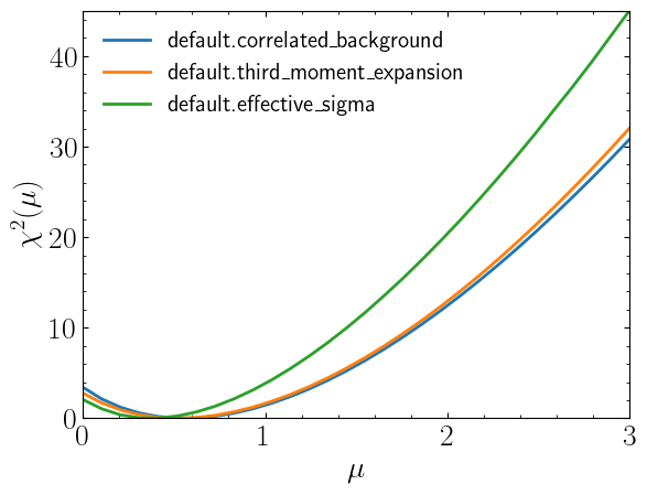
Comparing the Three Likelihood Prescriptions#

The three prescriptions — correlated background, third moment expansion, and effective sigma — differ in how they encode the asymmetry of background uncertainties. A natural way to compare them is via the chi-square function

\[ \chi^2(\mu) = -2\ln\Lambda(\mu) = -2\left[\ln\mathcal{L}(\mu, \hat{\hat{\boldsymbol{\theta}}}_\mu) - \ln\mathcal{L}(\hat{\mu}, \hat{\boldsymbol{\theta}})\right], \]

which is the profile likelihood ratio expressed in chi-square units. A horizontal cut at \(\chi^2 = 3.84\) (the 95th percentile of the \(\chi^2_1\) distribution) marks the boundary of the 95% confidence interval on \(\mu\); the corresponding \(\mu\) values are the upper limits. Differences between the three curves reflect the distinct treatment of uncertainty asymmetry in each model: the symmetric model (correlated background) will generally produce a broader chi-square parabola than the asymmetric models (third moment expansion and effective sigma) when the uncertainties are significantly skewed.

poi = np.linspace(0, 3, 30)

llhd = [corr_background_model.chi2(p) for p in poi]
llhd_tm = [third_mom_expansion_model.chi2(p) for p in poi]
llhd_es = [effective_sigma_model.chi2(p) for p in poi]

../_images/4f4affa6989188bd94debe98b19711ed010c4b6dd4976cf9fe30442cd27b7a36.png

Introduction to Spey: A Unified Statistical Inference Framework

Contents

Introduction to Spey: A Unified Statistical Inference Framework#

Motivation#

The Plugin Architecture#

Statistical Framework#

Profile Likelihood Ratio Test Statistic#

The CLs Method#

Asimov Dataset#

Experimental Data: CMS-SUS-20-004#

Simplified Likelihood: Correlated Background Model#

Profile Likelihood and Confidence Intervals#

Upper Limits and CLs Exclusion#

Third Moment Expansion#

Effective Sigma#

Comparing the Three Likelihood Prescriptions#