Signal Uncertainties

Let us assume that we have a set of signal uncertainties (such as scale and PDF uncertainties). We can extend the likelihood prescription to include these uncertainties as a new set of nuisance parameters.

Attention

Note that theoretical uncertainties have different interpretations, we can interpret them similar to experimental uncertainties, as we will do in this tutorial, or they can be interpreted as uncertainties on the cross-section. In the latter case one should compute the limits by changing the background uncertainties with respect to the change in cross section. Notice that the below example adds an extra source of error in terms of a normal distribution, this will widen the likelihood distribution. If this is not the intended use of the error source, it can be added as follows;

import spey
from math import sqrt

pdf_wrapper = spey.get_backend("default.uncorrelated_background")
statistical_model_sigunc = pdf_wrapper(
    signal_yields=[12.0],
    background_yields=[50.0],
    data=[36],
    absolute_uncertainties=[sqrt(12.0**2 + (12.0*0.2)**2)],
)

Notice that here we added 20% uncertainty on the signal yields.

Show code cell content

Hide code cell content

import spey
import numpy as np
import matplotlib.pyplot as plt

We can add uncorrelated signal uncertainties just like in uncorrelated background case

\[ \mathcal{L}(\mu, \theta) = \prod_{i\in{\rm bins}}{\rm Poiss}(n_i|\mu n^{(s)}_i + \theta_i^{(s)}\sigma^{(s)}_i + n^{(b)}_i + \theta_i^{(b)}\sigma^{(b)}_i) \cdot \prod_{j\in{\rm nui}}\mathcal{N}(\theta_j^{(b)}|0, 1) \cdot \prod_{j\in{\rm nui}}\mathcal{N}(\theta^{(s)}_j|0, 1)\ , \]

where \((s)\) superscript indicates signal and \((b)\) indicates background.

pdf_wrapper = spey.get_backend("default.uncorrelated_background")
statistical_model_sigunc = pdf_wrapper(
    signal_yields=[12.0, 15.0],
    background_yields=[50.0, 48.0],
    data=[36, 33],
    absolute_uncertainties=[12.0, 16.0],
    signal_uncertainty_configuration={"absolute_uncertainties": [3.0, 4.0]},
)

Similarly, we can construct signal uncertainties using "absolute_uncertainty_envelops" keyword which accepts upper and lower uncertainties as [(upper, lower)]. We can also add a correlation matrix with "correlation_matrix" keyword and third moments with "third_moments" keyword. Notice that these are completely independent of background. Now we can simply compute the limits as follows

print(f"1 - CLs: {statistical_model_sigunc.exclusion_confidence_level()[0]:.5f}")
print(f"POI upper limit: {statistical_model_sigunc.poi_upper_limit():.5f}")

1 - CLs: 0.96607
POI upper limit: 0.88808

Let us also check the \(\chi^2\) distribution with respect to POI which we expect the distribution should get wider with signal uncertainties. For this comparison we first need to define the model without signal uncertainties:

statistical_model = pdf_wrapper(
    signal_yields=[12.0, 15.0],
    background_yields=[50.0, 48.0],
    data=[36, 33],
    absolute_uncertainties=[12.0, 16.0],
)

Using statistical_model and statistical_model_sigunc we can compute the \(\chi^2\) distribution

Show code cell content

Hide code cell content

poi = np.linspace(-3,2,20)
plt.plot(poi, [statistical_model.chi2(p, allow_negative_signal=True) for p in poi], color="b", label="no signal uncertainties")
plt.plot(poi, [statistical_model_sigunc.chi2(p, allow_negative_signal=True) for p in poi], color="r", label="with signal uncertainties")
plt.legend()
plt.xlabel("$\mu$")
plt.ylabel("$\chi^2(\mu)$")
plt.show()

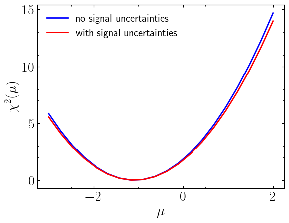
\(\chi^2(\mu)\) distribution comparisson for statistical model with and without signal uncertainties.