Exclusion limits

Any Spey statistical model can compute the exclusion confidence level using three different calculators. The availability of these options depends on the functions used in the likelihood construction (see this section for details).

The exclusion limits can be calculated for two different test statistic measure i.e. test statistic

\[\begin{split} q_\mu = \begin{cases} 0 & {\rm if\ } \hat{\mu}>\mu\ , \\ -2\log\frac{\mathcal{L}(\mu, \theta_\mu)}{\mathcal{L}(\hat{\mu}, \hat{\theta})} & {\rm otherwise} \end{cases} \quad , \end{split}\]

or alternate test statistic

\[\begin{split} \tilde{q}_\mu = \begin{cases} 0 & {\rm if\ } \hat{\mu}>\mu\ , \\ -2\log\frac{\mathcal{L}(\mu, \theta_\mu)}{\mathcal{L}(\hat{\mu}, \hat{\theta})} & {\rm if\ } 0\leq\hat{\mu}\leq\mu\ ,\\ -2\log\frac{\mathcal{L}(\mu, \theta_\mu)}{\mathcal{L}(0, \theta_0)} & {\rm otherwise} \end{cases}\quad . \end{split}\]

The main distinction being, alternate test statistic assumes that the signal can not be negative, for instance in case of negative interference effects in EFT one should use test statistic. By default exclusion_confidence_level() function assumes alternate test statistic being use and this can be changed with allow_negative_signal boolean argument.

Tip!

To check which calculators are available for a given model, users can call the available_calculators function.

The exclusion_confidence_level() function allows users to specify the calculator through the calculator keyword, offering three options:

How has the Asimov likelihood been calculated?

For exclusion limits, the first step is to fit the likelihood to the parameter of interest (POI) set to 0, representing the background-only model. Using the fitted parameters, expected data is generated, known as Asimov data. By replacing the observed data with this Asimov data, a new likelihood distribution—referred to as the “Asimov likelihood”—is created. This Asimov likelihood is then used for inference.

• “asymptotic”: Uses asymptotic formulae to compute p-values (see ref. [1] for details). This method requires the likelihood to support sampling capabilities, as it compares the signal-like test statistic to the Asimov test statistic using the formula \(t_\mu = \sqrt{\tilde{q}_\mu} - \sqrt{\tilde{q}_{\mu,A}}\). This is the most commonly used method in LHC analyses.

• “toy”: Relies on the likelihood’s sampling functionality. It calculates p-values by generating samples from both the signal-plus-background and background-only distributions.

• “chi_square”: Compares the signal hypothesis (\(\tilde{q}_{\mu=1}\)) to the null hypothesis, with the test statistic \(t_\mu = \sqrt{\chi^2(\mu=0)} - \sqrt{\tilde{q}_{\mu=1}}\). This approach was widely used during the Tevatron era.

The expected keyword allows users to select between computing observed or expected exclusion limits. It also supports the calculation of prefit expected exclusion limits, which can be enabled by setting expected=spey.ExpectationType.apriori. This option ignores experimental data and computes the expected exclusion limit based solely on the simulated Standard Model (SM) background yields. On the other hand, observed (for observed limits) and aposteriori (for post-fit expected limits) compute the exclusion confidence limits after fitting the model.

In both expected cases, the exclusion limits are returned with \(\pm1\sigma\) and \(\pm2\sigma\) variations around the background model, resulting in five values: \([-2\sigma, -1\sigma, 0, 1\sigma, 2\sigma]\). However, the observed exclusion limit returns a single value. The "chi_square" calculator is an exception—it only provides one value for both observed and expected limits.

The allow_negative_signal keyword controls which test statistic is used and restricts the values that \(\mu\) (the signal strength) can take when computing the maximum likelihood. When allow_negative_signal=True, the \(q_\mu\) test statistic is applied; otherwise, the \(\tilde{q}_\mu\) statistic is used (for further details, see [1, 2]).

For complex statistical models, optimizing the likelihood can be challenging and depends on the choice of optimizer. Spey uses SciPy for optimization and fitting tasks. Any additional keyword arguments not explicitly covered in the exclusion_confidence_level() function description are passed directly to the optimizer, allowing users to customize its behavior through the interface.

Below we compare the exclusion limits computed with each approach. This comparisson uses normal distribution for the likelihood (default.normal) background yields are set to \(n_b\), uncertainties are shown with \(\sigma\) and observations are given with \(n\).

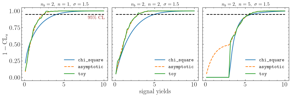
exclusion limit calculator comparisson for observed p-values

Example:

import spey

stat_wrapper = spey.get_backend("default.normal")
statistical_model = stat_wrapper(
    signal_yields=[3.0],
    background_yields=[2.0],
    absolute_uncertainties=[1.5],
    data=[2],
)

print(f"1-CLs value with calculator='asymptotic': {statistical_model.exclusion_confidence_level()[0]:.3f}")
print(f"1-CLs value with calculator='chi_square': {statistical_model.exclusion_confidence_level(calculator='chi_square')[0]:.3f}")
print(f"1-CLs value with calculator='toy': {statistical_model.exclusion_confidence_level(calculator='toy')[0]:.3f}")

1-CLs value with calculator='asymptotic': 0.954
1-CLs value with calculator='chi_square': 0.811
1-CLs value with calculator='toy': 0.965