Statistical inference on Histogram

In this tutorial, we will generate a mock histogram and see if our signal model is good enough to explain the experimental data.

Show code cell content

Hide code cell content

import numpy as np
import spey
import matplotlib.pyplot as plt

Let us generate a histogram to be used in our example first. In below example, we generate three sets of data, signal (\(n_s\)), background (\(n_b\)) and observarions (\(n\)). The statistical uncertainties on the background yields are shown with black lines.

Show code cell source

Hide code cell source

fig = plt.figure(figsize=(8, 6))
# Define the binning
nbins = 10
x = np.linspace(1, nbins, nbins)

# The background follows a linear shape
b_yields = np.array([(1 - i / 2 / nbins) for i in range(0, nbins)])
b_fracs = b_yields / np.sum(b_yields)

# The signal shape is a peak
s_fracs = np.zeros(nbins)
s_fracs[4:7] = [0.1, 0.8, 0.1]

# Define the signal and background
s = 3
b = 50
s_and_b = s * s_fracs + b * b_fracs
b_only = b * b_fracs

# Now generate some data for the s+b model
np.random.seed(14)
# Set the random seed to make sure we generate the same data every time
data = np.array(
    [
        np.random.poisson(s * s_frac + b * b_frac)
        for s_frac, b_frac in zip(s_fracs, b_fracs)
    ]
)

# Make a plot of the result
plt.bar(x, s_and_b, color="orange", label="signal and background")
plt.bar(
    x,
    b_only,
    color="b",
    label="background only",
    yerr=np.sqrt(b_only),
    capsize=3,
    error_kw={"lw": 1},
)
plt.scatter(x, data, zorder=10, color="k", label="data")
plt.xlabel("bin number")
plt.ylabel("Total expected yield")
plt.legend(fontsize=12)
plt.xlim([0.5, 10.5])
plt.show()

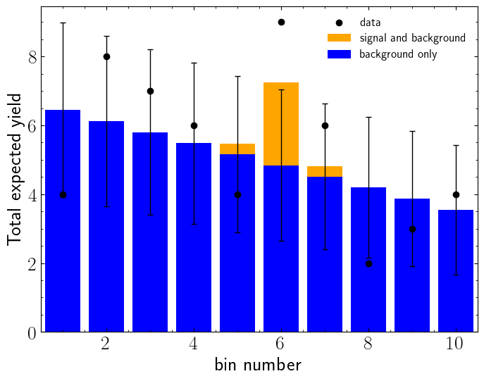
Lets construct a statistical model. Since the only source of uncertainty is statistical, we can safely assume that non of the bins are correlated in systematic level. Hence we will use "default.uncorrelated_background" model.

Tip!

In order to see the documentation for the wrapper, one can use ? syntax: pdf_wrapper?.

pdf_wrapper = spey.get_backend("default.uncorrelated_background")

stat_model = pdf_wrapper(
    signal_yields=s_and_b - b_only,
    background_yields=b_only,
    data=data,
    absolute_uncertainties=np.sqrt(b_only),
)

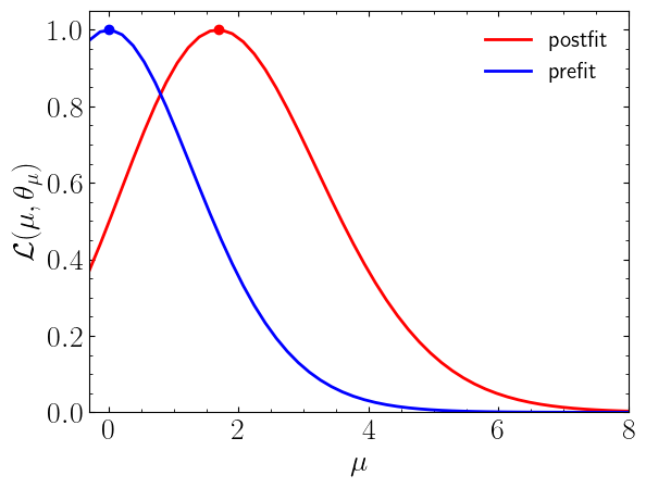
Now we can compute the normalised likelihood distribution for prefit and postfit statistical models.

Note

return_nll=False flag ensures that likelihood function returns the likelihood value instead of negative log-probability value.

poi = np.linspace(-0.3, 8, 50)

llhd_postfit = [stat_model.likelihood(p, return_nll=False) for p in poi]
muhat_postfit, max_llhd_postfit = stat_model.maximize_likelihood(return_nll=False)

llhd_prefit = [
    stat_model.likelihood(p, expected=spey.ExpectationType.apriori, return_nll=False)
    for p in poi
]
muhat_prefit, max_llhd_prefit = stat_model.maximize_likelihood(
    expected=spey.ExpectationType.apriori, return_nll=False
)

Show code cell source

Hide code cell source

plt.plot(poi, llhd_postfit / max_llhd_postfit, color="r", label="postfit")
plt.scatter(muhat_postfit, 1, color="r")

plt.plot(poi, llhd_prefit / max_llhd_prefit, color="b", label="prefit")
plt.scatter(muhat_prefit, 1, color="b")

plt.legend()

plt.ylabel(r"$\mathcal{L}(\mu,\theta_\mu)$")
plt.xlabel(r"$\mu$")
plt.xlim([-0.3, 8])
plt.ylim([0, 1.05])
plt.show()

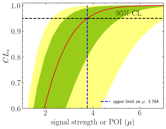
Now let us compute the expected and observed upper limits on signal strength (\(\mu\)) at 95% CL:

print(f"Observed upper limit on µ at 95% CL: {stat_model.poi_upper_limit():.5f}")

expected_pval = stat_model.poi_upper_limit(
    expected=spey.ExpectationType.aposteriori, expected_pvalue="1sigma"
)
muUL_apost = expected_pval[1]
print(
    "Expected upper limit on µ with ± 1σ at 95% CL: "
    + ",".join([f"{x:.3f}" for x in expected_pval])
)

Observed upper limit on µ at 95% CL: 4.66815
Expected upper limit on µ with ± 1σ at 95% CL: 2.834,3.764,5.183

We can use confidence_level flag to change the confidence level of our calculation

print(
    f"Observed upper limit on µ at 68% CL: {stat_model.poi_upper_limit(confidence_level=0.68):.5f}"
)

Observed upper limit on µ at 68% CL: 2.79069

Now let us compute the upper limit by hand:

poi = np.linspace(1, 7, 20)
poiUL = np.array(
    [
        stat_model.exclusion_confidence_level(
            poi_test=p, expected=spey.ExpectationType.aposteriori
        )
        for p in poi
    ]
)

Show code cell source

Hide code cell source

plt.plot(poi, poiUL[:, 2], color="tab:red")
plt.fill_between(poi, poiUL[:, 1], poiUL[:, 3], alpha=0.8, color="green", lw=0)
plt.fill_between(poi, poiUL[:, 0], poiUL[:, 4], alpha=0.5, color="yellow", lw=0)
plt.plot(
    [muUL_apost, muUL_apost],
    [0, 1],
    ls="dashed",
    color="b",
    label=f"upper limit on $\\mu$: {muUL_apost:.3f}",
)
plt.plot([0, 10], [0.95, 0.95], color="k", ls="dashed")
plt.xlabel(r"${\rm signal\ strength\ or\ POI }\ (\mu)$")
plt.ylabel("$CL_s$")
plt.xlim([1, 7])
plt.ylim([0.6, 1.01])
plt.text(5, 0.96, r"$95\%\ {\rm CL}$")
plt.legend(loc="lower right", fontsize=12)
plt.show()

Additionally we can compute the exclusion limit of our signal model to see if our model is excluded.

print(
    f"Observed exclusion confidence level, CLs: {stat_model.exclusion_confidence_level()[0]:.5f}"
)

exp_cls = stat_model.exclusion_confidence_level(expected=spey.ExpectationType.aposteriori)
print(
    f"Expected exclusion confidence level, CLs ± 1σ: {exp_cls[2]:.4f} - {exp_cls[2]-exp_cls[3]:.4f} + {exp_cls[1]-exp_cls[2]:.4f}"
)

Observed exclusion confidence level, CLs: 0.13942
Expected exclusion confidence level, CLs ± 1σ: 0.1620 - 0.0972 + 0.1182

Since our model is not excluded (\(1-{\rm CL}_s < 0.95\)), we may want to see the significance of our signal yields:

print(f"Z = {stat_model.significance()[1]:.3f}")

Z = 1.185