Difference between Spey & PyHf’s uncorrelated background models#

Both libraries provide a “simplest possible” single-channel counting model with a per-bin background uncertainty that is uncorrelated between bins. The construction at the surface looks the same, one Poisson term per bin plus a per-bin constraint on a nuisance parameter, but the type of constraint and how the nuisance parameter modifies the expected yield are different. This notebook makes the difference explicit, both mathematically and numerically.

1. Mathematical construction#

1.1 `"pyhf.uncorrelated_background"`#

pyhf builds the model with a shapesys modifier (see uncorrelated shape section). shapesys is a multiplicative modifier on the background sample, controlled by a nuisance parameter \(\gamma_i\) per bin which is constrained by a Poisson auxiliary measurement.

For a relative background uncertainty \(\sigma_i / n^b_i\), pyhf defines

\[ \alpha_i \;\equiv\; \frac{(n^b_i)^2}{\sigma_i^2} \]

and the full likelihood is

\[ \boxed{\; \mathcal{L}_{\text{pyhf}}(\mu, \boldsymbol{\gamma}) = \prod_{i=1}^{N} \mathrm{Poiss}\!\bigl(n^{\rm obs}_i \,\big|\, \mu n^s_i + \gamma_i n^b_i \bigr) \;\cdot\; \prod_{i=1}^{N} \mathrm{Poiss}\!\left(\alpha_i \,\big|\, \gamma_i\,\alpha_i\right) \;} \]

Key points:

The nuisance parameter \(\gamma_i\) is a multiplicative scale factor on the nominal background, with \(\gamma_i = 1\) at the SM point.
The constraint is Poisson with auxiliary observation \(\alpha_i = (n^b_i/\sigma_i)^2\) — i.e. the background uncertainty is treated as if it came from a control sample of effective size \(\alpha_i\).
Bounds are \(\gamma_i \in [10^{-10}, 10]\), so \(\gamma_i \ge 0\) is enforced by construction.

1.2 `"default.uncorrelated_background"`#

From the plug-ins section of the documentation the model is

\[ \boxed{\; \mathcal{L}_{\text{spey}}(\mu, \boldsymbol{\theta}) = \prod_{i=1}^{N} \mathrm{Poiss}\!\bigl(n^{\rm obs}_i \,\big|\, \mu n^s_i + n^b_i + \theta_i \sigma_i \bigr) \;\cdot\; \prod_{i=1}^{N} \mathcal{N}(\theta_i \mid 0, 1) \;} \]

Key points:

The nuisance parameter \(\theta_i\) is an additive pull in units of standard deviations: \(n^b_i \to n^b_i + \theta_i \sigma_i\).
The constraint is a standard normal centred at zero.
Positivity of \(n^b_i + \theta_i \sigma_i\) is not implicit; it is enforced explicitly during the fit via a scipy.optimize.NonlinearConstraint.

1.3 Reparametrisation: the two models are not identical#

Set \(\gamma_i = 1 + \theta_i \sigma_i / n^b_i\), then the Poisson mean in the main term becomes

\[ \gamma_i n^b_i = n^b_i + \theta_i \sigma_i \]

so the main models agree exactly. The constraint terms, however, differ:

Library	Constraint on \(\gamma_i \equiv 1 + \theta_i \sigma_i / n^b_i\)
pyhf	\(\mathrm{Poiss}\!\bigl(\alpha_i \mid \gamma_i \alpha_i\bigr)\) with \(\alpha_i = (n^b_i/\sigma_i)^2\)
spey	\(\mathcal{N}\!\bigl(\theta_i \mid 0, 1\bigr) = \mathcal{N}\!\bigl(\gamma_i \mid 1, \sigma_i/n^b_i\bigr)\)

By Stirling, \(\mathrm{Poiss}(\alpha \mid \gamma\alpha)\) around \(\gamma = 1\) behaves like \(\mathcal{N}(\gamma \mid 1, 1/\sqrt{\alpha}) = \mathcal{N}(\gamma \mid 1, \sigma/n^b)\). So in the large-\(\alpha\) (small relative uncertainty) limit the two constructions coincide. They diverge when \(\sigma_i / n^b_i\) is sizeable: the Poisson constraint is asymmetric in \(\gamma\) (heavier tail towards large \(\gamma\), hard floor at \(\gamma=0\)), while the Gaussian constraint is symmetric in \(\theta\) and assigns prior weight to \(n^b + \theta\sigma < 0\) which spey then forbids with a hard positivity wall.

2. Setup#

3. A toy single-bin scenario#

Single bin with \(n^s = 5\), \(n^b = 10\), \(\sigma = 4\), \(n^{\rm obs} = 11\). With \(\sigma/n^b = 40\%\) the relative uncertainty is large enough to see the Poisson/Gaussian mismatch.

signal = [5.0]
background = [10.0]
bkg_unc = [4.0]
data = [11]

pyhf_wrapper = spey.get_backend("pyhf.uncorrelated_background")
pyhf_model = pyhf_wrapper(
    signal_yields=signal,
    background_yields=background,
    data=data,
    absolute_uncertainties=bkg_unc,
)

print("pyhf parameters :", pyhf_model.config().parameter_names)
print(
    "pyhf auxdata    :",
    pyhf_model.backend.model()[-1][1],
    "= (n^b/sigma)^2 =",
    (background[0] / bkg_unc[0]) ** 2,
)
print("pyhf full data  :", pyhf_model.backend.model()[-1])

spey_wrapper = spey.get_backend("default.uncorrelated_background")
spey_model = spey_wrapper(
    signal_yields=signal,
    background_yields=background,
    data=data,
    absolute_uncertainties=bkg_unc,
)
print("spey backend    :", spey_model.backend.name)

pyhf parameters : ['mu', 'uncorr_bkguncrt[0]']
pyhf auxdata    : 6.25 = (n^b/sigma)^2 = 6.25
pyhf full data  : [11, 6.25]
spey backend    : default.uncorrelated_background

4. Compare the constraint terms directly#

Plot \(\ln \mathcal{C}_{\text{pyhf}}(\gamma)\) vs \(\ln \mathcal{C}_{\text{spey}}(\gamma)\) as a function of the same multiplicative scale \(\gamma = 1 + \theta\sigma/n^b\).

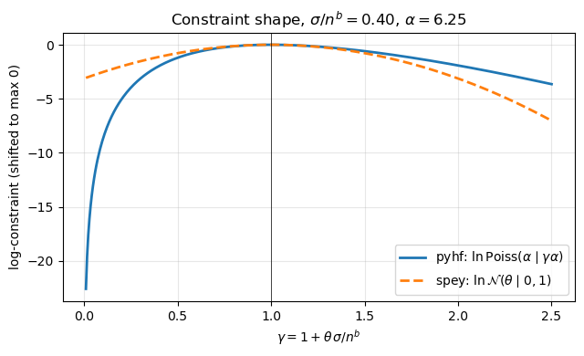
../_images/3bed6aea116a71df3fc8d027b15766178c2caf5d020980be6401e5beeb794e1a.png

Asymmetry of the pyhf Poisson constraint vs symmetric spey Gaussian:
  pyhf  log C at gamma=0.5 : -1.207
  pyhf  log C at gamma=1.5 : -0.591
  spey  log C at theta=-1  : -0.500
  spey  log C at theta=+1  : -0.500

The spey Gaussian is symmetric in \(\theta\), while the pyhf Poisson is skewed: it penalises downward fluctuations of the background more than upward ones. At small relative uncertainty the two curves overlap; at 40% they visibly disagree.

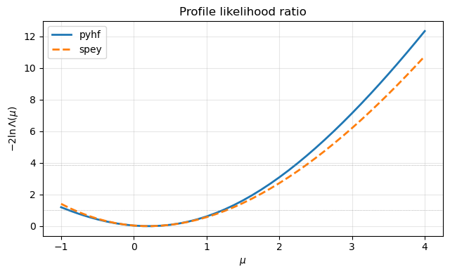
5. Profile likelihood ratio#

Profile out the nuisance parameter and compare \(-2 \ln \Lambda(\mu)\).

6. \(CL_s\) exclusion at \( \mu = 1\)#

excl_pyhf = float(pyhf_model.exclusion_confidence_level(poi_test=1.0)[0])
excl_spey = float(spey_model.exclusion_confidence_level(poi_test=1.0)[0])

print(f"pyhf  exclusion conf.    : {excl_pyhf:.4f}")
print(f"spey  exclusion conf.    : {excl_spey:.4f}")
print(f"difference (spey - pyhf) : {excl_spey - excl_pyhf:+.4f}")

pyhf  exclusion conf.    : 0.6235
spey  exclusion conf.    : 0.5759
difference (spey - pyhf) : -0.0476

7. Scaling: how the difference depends on \(\sigma / n^b\)#

Sweep the relative uncertainty. Small \(\sigma/n^b\): the two libraries should agree (Gaussian limit of Poisson). Large \(\sigma/n^b\): they should split.

rel_uncs = np.array([0.05, 0.10, 0.20, 0.30, 0.40, 0.60, 0.80])
results = []

for r in rel_uncs:
    sb_i = r * nb

    pm = pyhf_wrapper(
        signal_yields=signal,
        background_yields=background,
        data=data,
        absolute_uncertainties=[sb_i],
    )

    excl_p = float(pm.exclusion_confidence_level(poi_test=1.0)[0])

    sm = spey_wrapper(
        signal_yields=signal,
        background_yields=background,
        data=data,
        absolute_uncertainties=[sb_i],
    )
    excl_s = float(sm.exclusion_confidence_level(poi_test=1.0)[0])
    results.append((r, excl_p, excl_s))

results = np.array(results)
fig, ax = plt.subplots(figsize=(6.5, 4))
ax.plot(results[:, 0], results[:, 1], "o-", label="pyhf (1 - CLs)")
ax.plot(results[:, 0], results[:, 2], "s--", label="spey")
ax.set_xlabel(r"relative bkg uncertainty $\sigma/n^b$")
ax.set_ylabel(r"exclusion confidence at $\mu = 1$")
ax.set_title("Exclusion confidence vs relative background uncertainty")
ax.legend()
ax.grid(alpha=0.3)
plt.tight_layout()
plt.show()

pd.DataFrame(
    results, columns=["sigma/n_b", "exclusion (pyhf)", "exclusion (spey)"]
).round(4)

../_images/fd35cc3cb0beceb31c9262ca92dce2314203e439f8591f65a6284925a09138d9.png

	sigma/n_b	exclusion (pyhf)	exclusion (spey)
0	0.05	0.7703	0.7694
1	0.10	0.7604	0.7569
2	0.20	0.7249	0.7108
3	0.30	0.6764	0.6461
4	0.40	0.6235	0.5759
5	0.60	0.5239	0.4529
6	0.80	0.4427	0.3636

8. Summary#

Aspect	`pyhf` `uncorrelated_background`	`spey` `default.uncorrelated_background`
Modifier type	`shapesys` (multiplicative)	additive `theta * sigma`
Nuisance parameter	\(\gamma_i\), nominal \(\gamma_i = 1\)	\(\theta_i\), nominal \(\theta_i = 0\)
Effect on yield	\(\lambda_i = \mu n^s_i + \gamma_i n^b_i\)	\(\lambda_i = \mu n^s_i + n^b_i + \theta_i \sigma_i\)
Constraint	Poisson with auxdata \(\alpha_i = (n^b_i/\sigma_i)^2\)	Standard normal \(\mathcal{N}(0,1)\)
Positivity of \(n^b\)	guaranteed by \(\gamma_i \in [10^{-10}, 10]\)	enforced via `NonlinearConstraint` during fit
Symmetry of constraint	asymmetric in \(\gamma\)	symmetric in \(\theta\)
\(\sigma/n^b \ll 1\)	Stirling limit \(\to\) Gaussian	identical to pyhf
\(\sigma/n^b \gtrsim 0.3\)	skewed, harder downward penalty	symmetric pull

Bottom line. Under the reparametrisation \(\gamma_i = 1 + \theta_i\sigma_i/n^b_i\) the main Poisson term is identical in the two libraries. The difference is entirely in the constraint: pyhf uses an asymmetric Poisson constraint on the multiplicative scale, while spey’s default.uncorrelated_background uses a strictly Gaussian constraint on an additive pull. The discrepancy is invisible for small relative background uncertainties (small \(\sigma/n^b\), Stirling limit) and grows once \(\sigma/n^b\) exceeds \(\sim 30\%\), where the Poisson skewness becomes a real effect, visible above as the splitting of the two exclusion-confidence curves.

Use pyhf (or the spey-pyhf plugin that wraps it) when you need a Poisson-constrained uncorrelated background; use spey’s default.uncorrelated_background when you only have an absolute per-bin Gaussian uncertainty (typical for simplified likelihoods, arXiv:1809.05548)).

The reason for the differenfe is because in the HistFactory formalism that pyhf implements, shapesys is meant to model a statistical uncertainty on the background prediction and statistical uncertainties are Poisson by construction, not Gaussian.

The deeper reasoning has several threads:

The number \(\alpha_i = (n^b_i/\sigma_i)^2\) has a physical meaning. It is the effective sample size of the (real or MC) control region that produced the background prediction. If you imagine a control sample of \(\alpha_i\) events, scaled by a factor \(n^b_i / \alpha_i\) to produce the prediction \(n^b_i\), then the statistical uncertainty of that prediction is exactly \(\sqrt{\alpha_i} \cdot \frac{n^b_i}{\alpha_i} = \frac{n^b_i}{\sqrt{\alpha_i}} = \sigma_i.\) So shapesys is literally saying “the background in bin i was estimated from \(\alpha_i\) effective events”, and the auxiliary measurement is the Poisson count of those events. A Gaussian constraint would discard this interpretation.
Positivity is enforced for free. A Poisson constraint hard-zeros at \(\gamma_i = 0\). The expected background \(\gamma_i n^b_i\) literally cannot go negative. A Gaussian on \(\theta_i\) has nonzero prior mass at \(n^b_i + \theta_i \sigma_i < 0\), which is unphysical and is why spey has to bolt on an explicit NonlinearConstraint during optimisation. For low-statistics bins where \(\sigma_i / n^b_i\) is large, this matters numerically (it’s where the two constructions visibly disagree, as the notebook shows).
It’s the Barlow–Beeston-lite construction. shapesys is the same recipe Barlow & Beeston used for MC statistical uncertainties: one Poisson-constrained nuisance per bin, with the effective count interpreted as a control measurement. So this is consistent with how MC stats are treated everywhere else in HistFactory (staterror).
HistFactory has a clear convention. Stat-like uncertainties (shapesys, staterror) → Poisson constraint; systematic-like uncertainties (normsys, histosys) → Gaussian constraint. pyhf.uncorrelated_background chose shapesys because the natural interpretation of a per-bin background uncertainty with no further context is “stat error on the prediction”.
The Stirling limit gives you the Gaussian back when it’s appropriate. For high-stats bins (\(\alpha_i \gg 1\), equivalently \(\sigma_i / n^b_i \ll 1\)), Stirling turns the Poisson into a Gaussian with width \(\sigma_i\), so you lose nothing in the regime where Gaussian is a good description, and you keep the correct asymmetric tail in the regime where it isn’t.

So the difference is really a difference in intent: pyhf models a statistical control measurement; spey’s default.uncorrelated_background models a generic absolute Gaussian uncertainty (as in the simplified-likelihood prescription, arXiv:1809.05548).