Converting full statistical models to the simplified likelihood framework

A full pyhf HistFactory statistical model carries all the information necessary to reproduce an LHC analysis. The price to pay is that evaluating, profiling or sampling such a likelihood is often prohibitively expensive once the number of nuisance parameters grows into the hundreds, as is typical for ATLAS or CMS searches. The Simplify converter implemented in spey-pyhf projects a full likelihood onto a substantially cheaper simplified-likelihood form, in which a single combined nuisance parameter is retained for every analysis bin and all systematic uncertainties are summarised by the moments of the per-bin background distribution. Three target backends are supported:

• "default.correlated_background": Gaussian constraint with full bin-to-bin correlation;

• "default.third_moment_expansion": adds the leading skewness correction through a quadratic deformation of the expected counts;

• "default.effective_sigma": Barlow-style asymmetric Gaussian for skewed/bounded per-bin uncertainties.

Details on the simplified-likelihood backends themselves are given in the spey default plug-ins documentation.

This particular example requires the installation of three packages, which can be achieved with

>>> pip install spey spey-pyhf jax

The jax extra is required because the simplification algorithm queries the Hessian of the log-likelihood through automatic differentiation.

Methodology

The construction follows the simplified-likelihood framework of Buckley, Citron, Fichet, Kraml, Waltenberger and Wardle (JHEP 04 (2019) 064, arXiv:1809.05548), whose central result is that an experimental likelihood with \(N\) independent elementary nuisance parameters \(\boldsymbol{\delta}\) is well approximated, in the regime \(N \geq P\) where \(P\) is the number of analysis bins, by

(1)\[\mathcal{L}_S(\boldsymbol{\alpha}, \boldsymbol{\theta}) = \prod_{I=1}^{P} \mathrm{Pois}\!\left(n_I^{\mathrm{obs}} \,\big|\, n_{s,I}(\boldsymbol{\alpha}) + a_I + b_I \theta_I + c_I \theta_I^2 \right) \cdot \frac{\exp\!\left(-\tfrac{1}{2}\boldsymbol{\theta}^{\mathrm{T}} \boldsymbol{\rho}^{-1}\boldsymbol{\theta}\right)} {\sqrt{(2\pi)^P}} .\]

The \(P\) combined nuisance parameters \(\boldsymbol{\theta} = (\theta_1, \dots, \theta_P)\), one per bin, replace the much larger set of elementary \(\boldsymbol{\delta}\) and are unit-variance, centred Gaussians correlated through the \(P \times P\) matrix \(\boldsymbol{\rho}\). The coefficients \((a_I, b_I, c_I, \rho_{IJ})\) are obtained by matching the first three central moments of the per-bin background expectation \(\tilde{n}_b = a + b\theta + c\theta^2\) (at \(\mu = 0\)) to the corresponding moments of the full likelihood (Buckley et al. eqs. 2.6–2.8):

(2)\[\begin{split}m_{1,I} &= a_I + c_I , \\ m_{2,IJ} &= b_I b_J \rho_{IJ} + 2 c_I c_J \rho_{IJ}^{\,2} , \\ m_{3,I} &= 6\,b_I^{\,2} c_I + 8\,c_I^{\,3} .\end{split}\]

Inverting these relations (Buckley et al. eqs. 2.9–2.12) yields the simplified-likelihood parameters as closed-form functions of the moments:

(3)\[\begin{split}c_I &= -\mathrm{sign}(m_{3,I}) \sqrt{2\,m_{2,II}}\, \cos\!\left[ \frac{4\pi}{3} + \frac{1}{3}\, \arctan\!\sqrt{8\,\frac{m_{2,II}^{\,3}}{m_{3,I}^{\,2}} - 1} \right] , \\ b_I &= \sqrt{m_{2,II} - 2 c_I^{\,2}} , \\ a_I &= m_{1,I} - c_I , \\ \rho_{IJ} &= \frac{1}{4\,c_I c_J}\, \left(\sqrt{(b_I b_J)^2 + 8\,c_I c_J\,m_{2,IJ}} - b_I b_J\right) .\end{split}\]

These expressions are valid as long as \(8\,m_{2,II}^{\,3} \geq m_{3,I}^{\,2}\), i.e. the bin-wise skewness is small enough for the quadratic expansion to be invertible. When the third moment \(m_{3,I}\) vanishes the quadratic term drops out (\(c_I \rightarrow 0\)) and eq. (1) reduces to the standard simplified likelihood used by "default.correlated_background", with \(a_I = m_{1,I}\), \(b_I = \sqrt{m_{2,II}}\) and \(\rho_{IJ} = m_{2,IJ} / (b_I b_J)\), the Pearson correlation of \(\Sigma \equiv m_2\). The full quadratic form is implemented by "default.third_moment_expansion".

For asymmetric per-bin uncertainties the same combined-parameter strategy is used, but the linear term \(\theta_I\,\sigma_I\) in the expected count is replaced by Barlow’s variable-Gaussian prescription (arXiv:physics/0406120, Sec. 3.6):

(4)\[\sigma^{\mathrm{eff}}_I(\theta_I) = \sqrt{\sigma^{+}_I\,\sigma^{-}_I + (\sigma^{+}_I - \sigma^{-}_I)(\theta_I - n^{b}_I)} ,\]

so that the conditional standard deviation interpolates smoothly between the upper (\(\sigma^{+}\)) and lower (\(\sigma^{-}\)) absolute uncertainties of the bin. This is the form used by "default.effective_sigma"; when \(\sigma^{+} = \sigma^{-}\) the effective sigma reduces to the symmetric value and one recovers the standard simplified likelihood.

Extracting the moments from a pyhf model

In analyses where the analytical relationship between elementary and combined nuisance parameters is opaque, which is the typical case for pyhf workspaces, Buckley et al. Sec. 4 advocate extracting \((m_1, m_2, m_3)\) by Monte-Carlo. The Simplify converter realises this in five steps.

Step 1: Control likelihood. A control likelihood \(\mathcal{L}^{c}\) is built from the background-only pyhf workspace by attaching a zero-yield "Signal" sample to every channel listed in control_region_indices. The remaining channels keep their background-only structure. The parameter of interest \(\mu\) is retained in the workspace, but the resulting model has zero signal yields everywhere when \(\mu = 0\), so \(\mathcal{L}^{c}\) collapses to a background-only fit at that point. The control_region_indices argument selects the channels in which the (zero-valued) signal sample, and optionally the signal modifiers, are introduced, which controls whether signal-induced systematics enter the constraint covariance computed below.

Attention

The shape of \(\boldsymbol{\rho}\), and thus the quality of the simplification, depends sensitively on which channels are declared as control/validation regions and on whether the signal modifiers are propagated. Channels in which a potential signal overlaps with the background fit can bias the nuisance MLE; the convention adopted here, following the original simplified-likelihood proposal, is to compute the nuisance covariance from regions that are expected to be signal-free or signal-depleted.

Step 2: Conditional MLE. \(\mathcal{L}^{c}\) is profiled at \(\mu = 0\) to obtain the conditional best-fit nuisance vector \(\hat{\boldsymbol{\theta}}_0^{c}\). This is the maximum-likelihood point of the background-only fit consistent with no signal contribution.

Step 3: Nuisance covariance. Once \(\hat{\boldsymbol{\theta}}_0^{c}\) is found, the observed Fisher information is read off the Hessian of the negative log-likelihood,

(5)\[V^{-1}_{ij} = -\,\frac{\partial^{2} \log\mathcal{L}^{c}}{\partial\theta_i\,\partial\theta_j} \bigg|_{(\mu,\,\boldsymbol{\theta}) = (0,\,\hat{\boldsymbol{\theta}}_0^{c})} ,\]

where the row and column corresponding to \(\mu\) are removed before the inversion. The resulting matrix \(\mathbf{V}\) is the asymptotic covariance of the nuisance parameters at the conditional MLE, and it captures all linear correlations between them.

Step 4: Nuisance sampling. A multivariate Gaussian \(\mathcal{N}(\hat{\boldsymbol{\theta}}_0^{c}, \mathbf{V})\) is constructed, and nuisance draws \(\tilde{\boldsymbol{\theta}} \sim \mathcal{N}(\hat{\boldsymbol{\theta}}_0^{c}, \mathbf{V})\) are sampled from it without losing the correlations between elementary nuisance parameters.

It is important to note that the nuisance parameters of \(\mathcal{L}^{c}\) need not match exactly those of the requested full statistical model \(\mathcal{L}^{\mathrm{SR}}\), which may carry additional modifiers that are absent from the control regions. When \(|\boldsymbol{\theta}^{\mathrm{SR}}| > |\tilde{\boldsymbol{\theta}}^{c}|\) the missing entries are profiled by maximising \(\mathcal{L}^{\mathrm{SR}}\) at \(\mu = 0\) with the shared entries held at \(\tilde{\boldsymbol{\theta}}^{c}\) through equality constraints. The resulting maximiser \(\hat{\boldsymbol{\theta}}^{\mathrm{SR}}\) together with \(\tilde{\boldsymbol{\theta}}^{c}\) provides a complete nuisance vector that can be evaluated on \(\mathcal{L}^{\mathrm{SR}}\).

Step 5: Per-bin sampling. Each accepted parameter vector is forwarded to the pyhf sampler of \(\mathcal{L}^{\mathrm{SR}}\) to draw one Poisson realisation per bin,

(6)\[\tilde{n}_b \sim \mathcal{L}^{\mathrm{SR}}\!\left(\mu = 0,\, \tilde{\boldsymbol{\theta}}^{c},\, \hat{\boldsymbol{\theta}}^{\mathrm{SR}}\right) ,\]

with the auxiliary data deliberately excluded so that the resulting samples encode only the per-bin background expectation propagated through the nuisance fluctuations. Samples that would require drawing from a Poisson with non-positive rate are rejected and the loop continues until number_of_samples accepted samples are collected.

Estimating the moments. Given the matrix of samples, the simplified-likelihood inputs are obtained as

\[\begin{split}m_1 &= \mathbb{E}[\tilde{n}_b] , \\ \Sigma &\equiv m_2 = \mathrm{cov}(\tilde{n}_b) , \\ m_3 &= \mathbb{E}\!\left[(\tilde{n}_b - m_1)^3\right] .\end{split}\]

The per-bin background expectation passed to the simplified-likelihood backend is therefore the sample mean \(m_1\), not the original yield from the pyhf workspace, the simplified framework treats \(m_{1,I}\) as the first moment of the bin distribution. For “default.effective_sigma” the \((m_1, \Sigma)\) summary is supplemented by the 68% sample quantiles that define the per-bin asymmetric envelope,

\[\begin{split}\sigma^{+}_I &= |\,Q_{0.8413}(\tilde{n}_{b,I}) - m_{1,I}\,| , \\ \sigma^{-}_I &= |\,m_{1,I} - Q_{0.1587}(\tilde{n}_{b,I})\,| ,\end{split}\]

where \(Q_p\) denotes the empirical \(p\)-quantile (the \(\pm 1\sigma\) quantiles of a standard normal). The covariance \(\Sigma\) is then reduced to the corresponding Pearson correlation matrix \(\rho_{IJ} = \Sigma_{IJ}/\sqrt{\Sigma_{II}\,\Sigma_{JJ}}\), which is passed to “default.effective_sigma” together with the asymmetric envelope.

Note

Possible leakage of signal into control or validation regions is disregarded by setting the signal yields to zero while constructing \(\mathcal{L}^{c}\). The per-bin samples \(\tilde{n}_b\) are drawn without auxiliary data, hence the resulting simplified statistical model contains a single nuisance parameter per bin summarising all systematic uncertainties.

See also

Other techniques have been employed to simplify full statistical models. One example is the eschanet/simplify tool, which produces a pyhf-compatible JSON patch by collapsing the post-fit background of a workspace into a single sample. Its output can be loaded directly with the spey-pyhf plug-in without additional modifications. The approach implemented here is different in that it samples the full likelihood and matches moments of the resulting per-bin distribution rather than freezing nuisance parameters at their post-fit values.

Usage

A full statistical model can be constructed using a background-only JSON-serialised file (typically found in the HEPData entry for a given analysis). Details on constructing a full likelihood through the spey-pyhf interface can be found in this section.

As an example, let us use the JSON files provided for the ATLAS-SUSY-2019-08 analysis on HEPData. The files can be read using the standard json module:

>>> import json
>>> with open("1Lbb-likelihoods-hepdata/BkgOnly.json", "r") as f:
>>>     background_only = json.load(f)
>>> with open("1Lbb-likelihoods-hepdata/patchset.json", "r") as f:
>>>     signal = json.load(f)["patches"][0]["patch"]

Following the details in the previous sections, a statistical model using the pyhf interface can be constructed as

>>> import spey
>>> pdf_wrapper = spey.get_backend("pyhf")
>>> full_statistical_model = pdf_wrapper(
...     background_only_model=background_only, signal_patch=signal
... )
>>> full_statistical_model.backend.manager.backend = "jax"

where background_only is the background-only JSON file retrieved from HEPData and signal is a signal patch. The last line enables pyhf’s jax backend, which is required for the Hessian computation in eq. (5). full_statistical_model can then be converted into a simplified likelihood with the pyhf.simplify backend:

>>> converter = spey.get_backend("pyhf.simplify")
>>> simplified_model = converter(
...     statistical_model=full_statistical_model,
...     convert_to="default.correlated_background",
...     control_region_indices=[
...         'WREM_cuts', 'STCREM_cuts', 'TRHMEM_cuts', 'TRMMEM_cuts', 'TRLMEM_cuts'
...     ]
... )

Arguments: (for details see the object reference for Simplify)

• statistical_model: full statistical model constructed using the pyhf backend with the jax backend enabled.

• fittype: which expectation type is used when constructing and profiling the control model. "postfit" uses the observed auxiliary data, "prefit" uses the pre-fit auxiliary data.

• convert_to: target simplified-likelihood backend, one of "default.correlated_background", "default.third_moment_expansion" or "default.effective_sigma". Default is "default.correlated_background".

• number_of_samples: number of accepted Monte-Carlo samples used to estimate \(m_1\), \(\Sigma\) (and where relevant \(m_3\) or the asymmetric quantile envelope). Default 1000.

• control_region_indices: indices or names of the control and validation regions in the background-only workspace. The algorithm includes a substring-based heuristic that detects channel names containing CR or VR, but the convention varies between collaborations and the heuristic can fail. The channel names of the statistical_model can be read from list(statistical_model.backend.model.channels); see channels.

• include_modifiers_in_control_model: when True, the signal modifiers are attached to the zero-yield signal samples injected into the control regions, so that signal-induced systematics contribute to \(\mathbf{V}\) in eq. (5). Default False.

Saving and restoring the simplified model

The Monte-Carlo extraction is the most expensive step of the conversion. To avoid having to repeat it, the save_model argument of Simplify writes the extracted summary statistics to a compressed NumPy archive that can be reloaded with numpy.load(). The archive always contains the channel order, the per-bin observed data, the per-bin sample mean (the simplified-likelihood background yields \(m_{1,I}\)) and the per-bin covariance matrix \(\Sigma\); for "default.third_moment_expansion" it additionally contains the diagonal third moments \(m_{3,I}\), and for "default.effective_sigma" the asymmetric envelopes \((\sigma^{+}_I, \sigma^{-}_I)\).

Validation

Following the example above, we converted the full likelihood provided for the ATLAS-SUSY-2019-08 analysis into the "default.correlated_background" model (see the dedicated documentation for the target model). The results below use all available channels in the control model and include the modifiers of the signal patchset inside the control model. The postfit configuration is used throughout the simulation. The background yields and covariance matrix of the background-only model were computed from 500 samples drawn from the full statistical model. The scan includes 67 randomly chosen points in the \((m_{\tilde{\chi}^\pm_1/\tilde{\chi}^0_2},\,m_{\tilde{\chi}_1^0})\) mass plane.

The following plot shows the observed exclusion limit comparison between the full statistical model and its simplified version mapped onto the "default.correlated_background" backend. Data points only include those provided by the ATLAS collaboration on HEPData.

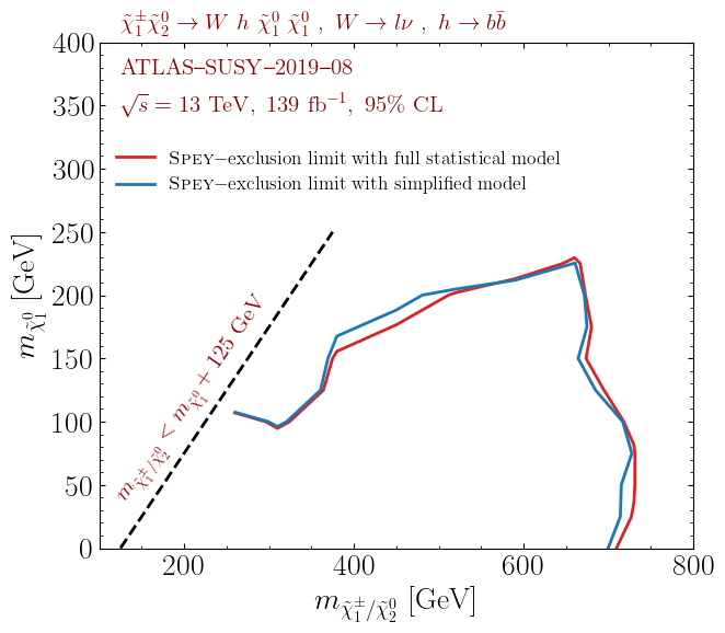
These results can be reproduced by following the prescription above. Note that the red curve does not correspond to the official results, because it is plotted from only 67 mass points; the official limit can be reproduced using the full patch set provided by the collaboration.

Comparison with pyhf’s in-house simplification tool

The eschanet/simplify tool (eschanet/simplify; see also the ATLAS PUB note ATL-PHYS-PUB-2021-038) implements an alternative path from a pyhf HistFactory workspace to a compact statistical model. Because its output is itself a pyhf workspace, it can be loaded directly through the spey-pyhf interface without going through the converter described in this page. The two methods solve the same problem, trading the long list of elementary nuisance parameters for one bin-wise uncertainty source, but the simplifications they apply are different and lead to different statistical models. The comparison below is intended to make the differences explicit so that users can pick the approximation that matches their use case.

Reference setup

Let \(\nu_I(\boldsymbol{\theta})\) denote the per-bin total expected count of the full pyhf model, where \(\boldsymbol{\theta} = (\theta_1, \dots, \theta_N)\) collects all elementary nuisance parameters. After fitting the full model one obtains the maximum-likelihood estimate \(\hat{\boldsymbol{\theta}}\) and the corresponding parameter covariance \(\mathbf{C} \in \mathbb{R}^{N\times N}\) (with \(\sigma_i \equiv \sqrt{C_{ii}}\) and Pearson correlation \(r_{ij} = C_{ij}/(\sigma_i\sigma_j)\)). The two methods use this information differently.

eschanet/simplify: post-fit linearised error propagation

For every parameter \(\theta_i\) the implementation computes a symmetric finite-difference variation of the per-bin expectation:

(7)\[\Delta_{I,i} = \frac{ \nu_I\!\left(\hat{\boldsymbol{\theta}} + \sigma_i\,\hat{e}_i\right) - \nu_I\!\left(\hat{\boldsymbol{\theta}} - \sigma_i\,\hat{e}_i\right) }{2} ,\]

with \(\hat{e}_i\) the unit vector along \(\theta_i\). In the limit of small \(\sigma_i\) this is exactly the first-order Taylor coefficient \(\Delta_{I,i} \simeq \sigma_i\,\partial\nu_I/\partial\theta_i\). The total per-bin variance is then obtained by linearised error propagation through the post-fit correlation matrix:

(8)\[\sigma_{b,I}^{2} = \sum_{i=1}^{N} \Delta_{I,i}^{\,2} + 2 \sum_{i>j} r_{ij}\,\Delta_{I,i}\,\Delta_{I,j} ,\]

equivalent in matrix form to \(\sigma_{b,I}^{2} = \boldsymbol{\Delta}_{I}^{\mathrm{T}}\, \mathbf{R}\,\boldsymbol{\Delta}_{I}\), where \(\mathbf{R}\) is the post-fit correlation matrix and \(\boldsymbol{\Delta}_{I}\) is the column vector of finite-difference slopes for bin \(I\). Pairs of pure staterror parameters are treated as uncorrelated by convention.

The output workspace contains one channel per surviving channel of the original model, each with a single "Bkg" sample whose nominal yield is the post-fit prediction \(\nu_I(\hat{\boldsymbol{\theta}})\) and a single histosys modifier named totalError with templates

(9)\[\nu^{\pm}_{I} = \nu_I(\hat{\boldsymbol{\theta}}) \pm \sigma_{b,I} .\]

The likelihood evaluated on this workspace is, schematically,

(10)\[\mathcal{L}_{\mathrm{esh}}(\mu, \boldsymbol{\theta}) = \prod_{I=1}^{P} \mathrm{Pois}\!\left(n_I^{\mathrm{obs}} \,\big|\, \mu\,n^{s}_I + \nu_I(\hat{\boldsymbol{\theta}}) + \sigma_{b,I}\,\theta_I^{\mathrm{tot}}\right) \cdot \prod_{I=1}^{P}\mathcal{N}\!\left(0\,\big|\,\theta_I^{\mathrm{tot}},\,1\right) ,\]

where each \(\theta_I^{\mathrm{tot}}\) is the nuisance parameter associated with the totalError modifier of bin \(I\) and the histosys interpolation provides the linear morphing between \(\nu_I\) and \(\nu^{\pm}_{I}\) consistent with eq. (9).

spey-pyhf.simplify: Monte-Carlo moment extraction

The converter implemented here, by contrast, samples \(\tilde{\boldsymbol{\theta}}\) from the constraint \(\mathcal{N}(\hat{\boldsymbol{\theta}}_0^{c}, \mathbf{V})\) and propagates each draw through the full likelihood before estimating the moments of the resulting per-bin distribution:

(11)\[\begin{split}m_{1,I} &= \mathbb{E}\!\left[\,\nu_I(\tilde{\boldsymbol{\theta}})\,\right] , \\ m_{2,IJ} &= \mathrm{cov}\!\left[\,\nu_I(\tilde{\boldsymbol{\theta}}),\, \nu_J(\tilde{\boldsymbol{\theta}})\,\right] , \\ m_{3,I} &= \mathbb{E}\!\left[\, \left(\nu_I(\tilde{\boldsymbol{\theta}}) - m_{1,I}\right)^{3}\,\right] .\end{split}\]

These moments feed eqs. (2) and (3) to produce the CorrelatedBackground or ThirdMomentExpansion simplified likelihood, eq. (1). The mapping is fully described in Methodology above; for the asymmetric variant the Barlow effective-\(\sigma\), eq. (4), is used instead.

Side-by-side

The following table summarises the differences.

Aspect	eschanet/simplify	spey-pyhf.simplify
Order of approximation	First-order Taylor expansion of \(\nu_I(\boldsymbol{\theta})\) around \(\hat{\boldsymbol{\theta}}\), eq. (7).	Non-linear propagation through Monte-Carlo: full evaluation of \(\nu_I(\tilde{\boldsymbol{\theta}})\) for each draw, eq. (11).
Where the fit is performed	Global fit of the full likelihood (signal + background, or background-only).	Background-only profile of a control likelihood \(\mathcal{L}^{c}\) at \(\mu = 0\), eq. (5).
Parameter covariance source	Post-fit covariance \(\mathbf{C}\) from MINUIT (HESSE) on the full model.	Observed Fisher information \(\mathbf{V}\) evaluated via JAX automatic differentiation on \(\mathcal{L}^{c}\), eq. (5).
Per-bin uncertainty	Symmetric Gaussian: \(\sigma_{b,I}^{2} = \boldsymbol{\Delta}_{I}^{\mathrm{T}} \mathbf{R}\,\boldsymbol{\Delta}_{I}\), eq. (8).	First two (optionally three) central moments \((m_{1,I}, m_{2,II}, m_{3,I})\), or the empirical 68 % quantiles for “default.effective_sigma”.
Bin-to-bin correlation	Absent. Each bin receives an independent histosys constraint with unit-width Gaussian prior; off-diagonal \(m_{2,IJ}\) information is dropped.	Retained in \(m_{2,IJ}\) and propagated to the multivariate-Gaussian constraint \(\boldsymbol{\theta} \sim \mathcal{N}(\mathbf{0},\boldsymbol{\rho})\).
Skewness / asymmetry	Not represented; the variable-Gaussian envelope is symmetric.	Optional via \(m_{3,I}\), eqs. (2) and (3), or via the asymmetric quantile envelope \((\sigma^{+}_I, \sigma^{-}_I)\) of eq. (4).
Treatment of staterror×staterror correlations	Forced to zero, regardless of the entry of \(\mathbf{R}\).	Preserved through the Hessian of \(\mathcal{L}^{c}\) and the multivariate-Gaussian sampling.
Output format	A pyhf HistFactory JSON patch (one Bkg sample plus one histosys modifier per channel) consumable by any pyhf front-end.	A native spey simplified-likelihood model (CorrelatedBackground, ThirdMomentExpansion or "default.effective_sigma").
Dominant computational cost	\(\mathcal{O}(N)\) evaluations of \(\nu_I\) (one symmetric pair per nuisance parameter).	\(\mathcal{O}(M)\) full-model evaluations, where \(M\) is number_of_samples, plus one Hessian.

Relationship in a common limit

In the regime where the post-fit log-likelihood is well approximated by a multivariate Gaussian in \(\boldsymbol{\theta}\), both methods estimate the same first two moments of \(\nu_I(\boldsymbol{\theta})\). Indeed, linearising \(\nu_I(\boldsymbol{\theta}) \simeq \nu_I(\hat{\boldsymbol{\theta}}) + \mathbf{g}_I^{\mathrm{T}} \delta\boldsymbol{\theta}\) with \(\mathbf{g}_{I,i} \equiv \partial\nu_I/\partial\theta_i\) and sampling \(\delta\boldsymbol{\theta} \sim \mathcal{N}(0, \mathbf{C})\) gives

(12)\[m_{1,I} \xrightarrow{\text{linear}} \nu_I(\hat{\boldsymbol{\theta}}) , \qquad m_{2,IJ} \xrightarrow{\text{linear}} \mathbf{g}_I^{\mathrm{T}} \mathbf{C}\, \mathbf{g}_J \;=\; \sum_{i,j} C_{ij}\, \frac{\partial\nu_I}{\partial\theta_i}\, \frac{\partial\nu_J}{\partial\theta_j} , \qquad m_{3,I} \xrightarrow{\text{linear}} 0 .\]

The eschanet/simplify per-bin variance, eq. (8), is precisely the diagonal \(I = J\) of this expression with the gradients replaced by central finite differences. The two approaches therefore coincide on the diagonal of \(m_2\), up to the discretisation of the finite difference and the choice of fit (control vs. global), when the model is locally linear in \(\boldsymbol{\theta}\) and the elementary nuisance parameters are jointly Gaussian. They part ways whenever any of the following is non-negligible:

• Non-linearity in \(\nu_I(\boldsymbol{\theta})\) (e.g. histosys interpolation outside the linear regime, large normsys shifts, log-normal lumi-style modifiers): the Taylor expansion drops \(\mathcal{O}(\delta\theta^2)\) corrections that the Monte-Carlo retains exactly.

• Bin-to-bin correlation: only the off-diagonal \(m_{2,IJ}\) retained by spey-pyhf couples bins; eschanet/simplify decouples them by construction.

• Skewness / boundedness: positivity of yields, asymmetric histosys templates, or visibly skewed post-fit distributions generate non-zero \(m_{3,I}\) and asymmetric quantiles that "default.third_moment_expansion" and "default.effective_sigma" use, but that eschanet/simplify discards.

Which approximation to use therefore depends on whether bin correlations and higher-order effects matter for the analysis at hand. When they do not, the lightweight pyhf patch produced by eschanet/simplify is sufficient; when they do, the moment-based reduction implemented here preserves the relevant information at the cost of an additional Monte-Carlo pass.

References

• A. Buckley, M. Citron, S. Fichet, S. Kraml, W. Waltenberger and N. Wardle, The Simplified Likelihood Framework, JHEP 04 (2019) 064, arXiv:1809.05548. Defines the simplified likelihood, the moment-matching parameters and the Monte-Carlo extraction procedure used here.

• R. Barlow, Asymmetric Errors, arXiv:physics/0406120, Sec. 3.6. Source of the variable-Gaussian effective-\(\sigma\) form consumed by “default.effective_sigma”.

• E. Schanet, simplify package (eschanet/simplify). Complementary tool that emits a pyhf-compatible JSON patch by freezing the post-fit background into a single sample.

Acknowledgements

This functionality has been discussed and requested during the 8th (Re)interpretation Forum. Thanks to Nicholas Wardle, Sabine Kraml and Wolfgang Waltenberger for the lively discussion.